Survival analysis is a branch of statistics for analyzing the expected duration of time until one or more events happen.  It has a very wide range of applications, such as death in biological organisms, failure in mechanical systems, reliability research for business, criminology, social and behavioral sciences and so on.

Special in SPSS

·  Classic Survival Analysis Fully Supported:

All Classic Survival Analysis methods are fully supported within one algorithm package.

·  PMML File Output:

This feature helps to separate the model building and the predicting. By storing the model in a PMML file scoring can be done later. This is a common feature for SPSS model building algorithms.

Survival Analysis Available in these Products

 Product integration with UI

• SPSS Statistics 25.0.0 Contains part of the Survival analysis component methods, such as Cox and, Kaplan-Meier

Spark and Python APIs

• IBM Watson Studio
• IBM SPSS Algorithm Spark and Python API

Survival Analysis can handle two kinds of data sets:

* Survival Data: regular survival analysis data that are non-recurrent: a single survival time is of interest for each subject.

• Time: information on duration to failure. 
• Frequency: is the frequency count, characterizing how many such records exist in the data set.
• Predictors: the factors which may impact the survival time by some degree.
• Status: the censored status of a record.

 * Recurrent Data: In some applications, events of interest may happen multiple times for each subject. Data recording such information are called recurrent data.

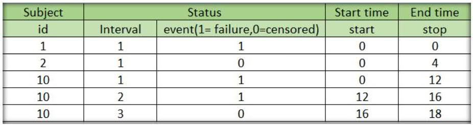
• Each line of data for a given subject lists the start time and stop time for each interval of follow-up.
• Different subjects are not restricted to have the same number of time intervals. Also they can have different start time and stop times.

The difference between regular survival analysis data and recurrent data is that the regular data only use one ID to identify one record. But in recurrent data, the Subject id and interval ID are both necessary for identifying different records.

The IBM SPSS Survival Analysis Algorithm allows input data with the conditions below:

1. For survival data, not having complete time information records within the whole life cycle, time information records may be lost at the beginning of the survey, during the survey or after the survey. Those data “lost” are called “censored”.


SPSS allows user input data which have:

• Uncensored Data - Complete data, the value of each sample unit is observed or known.

•       Right Censored Data - A data point goes beyond a certain time value but it is unknown by how much.

For example, if we tested five units and only three had failed by the end of the test, we would have right censored data (or suspension data) for the two units that did not fail. The term right censored implies that the event of interest is to the right of our data point.

In other words, if the units were to keep on operating, the failure would occur at some time after our data point.

•       Interval Censored Data - A data point is somewhere on an interval between two values.

For example, if we are running a medical equipment test on five units and inspecting them every 100 hours, we only know that a unit failed or did not fail between inspections. Specifically, if we inspect a certain unit at 100 hours and find it operating, and then perform another inspection at 200 hours to find that the unit is no longer operating, then the only information we have is that the unit failed at some point in the interval between 100 and 200 hours. This type of censored data is also called inspection data.

•       Left Censored Data - A data point is below a certain value but it is unknown by how much.

The left censored data may have some similar points with Interval censored data. Left censored data is identical to interval censored data whose starting time is zero.

For instance, as with the example above for Interval censored data, the left censored data have a certain unit failing sometime before 100 hours but it is not known exactly when. In other words, it could have failed any time between 0 and 100 hours.

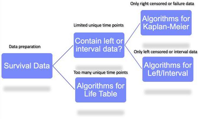
Roughly, a user could select which SPSS Survival analysis method to use by following the chart below:

2. For recurrent data, SPSS could handle the two kinds of data sets below:

•      Uncensored Recurrent Data
•      Right Censored Recurrent Data

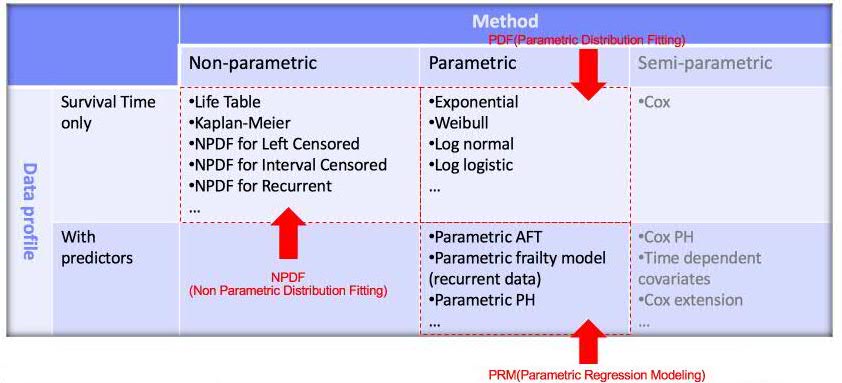
Based on data structure and the problem that users want to resolve, there are three kinds of methods for survival analysis: non-parametric, parametric and semi-parametric. They can be further divided by the presence or absence of predictors.

Details of the data type and analysis method are shown in this table:

By using the above methods, a user could:

• Get a lifetime table for survival data.
• Get the relationship between a specified field and survival time.
• Predict survival at regular intervals, predict survival at times specified by a variable and calculate the hazard function.

Algorithm Introduction

The IBM SPSS algorithm applies three kinds of survival analysis methods:

1. Non-Parametric Distribution Fitting(NPDF) – suitable for non-parametric survival analysis without predictors

• Input Data

• • Survival time (one or two fields).
  • Status (Failure or Right Censored, Left Censored, Interval Censored).
  • Allowed left truncation time field.
  • Groups and strata.
  • Additional fields for recurrent data.

• Output Objectives
  • First compute the distribution of survival times.
  • Carry out a test for group similarity/dissimilarity for each, or across, strata.

      For Example:

      A pharmaceutical company is developing an anti-inflammatory medication for treating chronic arthritic pain. Of particular interest is the time it takes for the drug to take effect and how it compares to an existing medication. They would like to know whether the new drug can improve over the traditional therapy and identify a group of similar medications. The result will suggest them how to create their future action plan.

Here are the data they collected.

In this data:

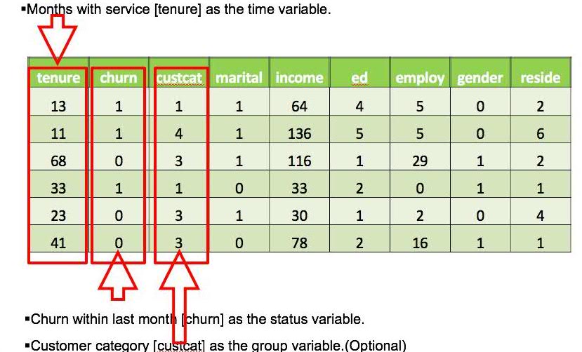
• time. The time at which the event or censoring occurred. The time variable should be continuous.
• status. Indicates whether the case experienced a terminal event(0) or was censored(1). The status variable can be categorical or continuous.
• Factor. Select a factor variable to examine group differences. Factor variables should be categorical if existed.
• Strata . Select a strata variable which will produce separate analyses for each level (stratum) of the variable. Strata variables should be categorical if they existed.

For this data, we can select the Kaplan- Meier method as in SPSS Statistics and indicate fields as shown below:  

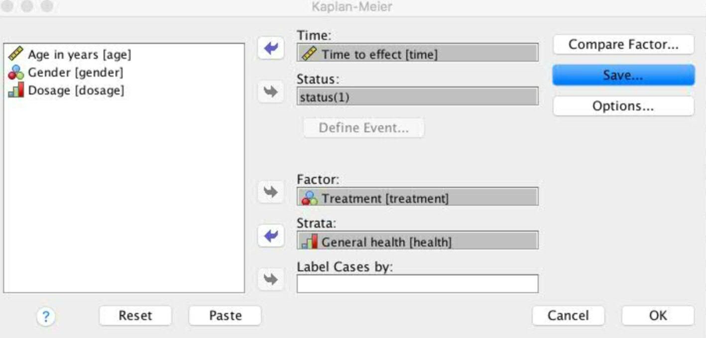
Select “treatment” as the factor to separate the different drugs being used for the patients, grouped by different patients’ health status (“health”). After building the model, it will show a life table like that shown below:

From the chart, we can see that when the patient health condition is poor,  the plot for the existing drug goes below that of the new drug most of the time. In other words, given a cum. survival value, most of the time the new drug requires more "time to effect" then the existing drug which suggests that the existing drug may give faster relief than the new. 

Correspondingly we can also get the other health condition charts below:

From above two charts, we can see that the plot for the New drug goes below that of the Existing drug throughout most of the trial, which suggests that the new drug may give faster relief than the old.   

By checking the test of equality of survival distributions for the different levels of Treatments as shown below, we can see that the significance values of the tests are all greater than 0.05, the comparison tests show that there is not a statistically significant difference between the New Drug and the Existing Drug.

So the final conclusion from this model is that new drug is highly recommended especially for poor health condition people since it will take effect faster than the old drug for them .

2. Parametric Distribution Fitting(PDF) – suitable for the Parametric survival analysis without predictors

• Input Data
  
  • Survival time (one or two fields).
  • Status (Failure or Right Censored, Left Censored, Interval Censored).
  • Allowed left truncation time field.
  • Groups.

• Output Objectives
  
  • Compute parametric distribution of survival times.
  • Carry out Goodness of fit test to judge if we fit the distribution well.
  • Compute Group Comparison for similarity/dissimilarity around each group.

 For Example:

A telecommunications company is interested in the issue of how long their customers are more likely to churn. The company wants to model the time to churn, in order to figure out how all the factors influence the “time to churn”.

     
      The company provides data as follows:

In this case, besides the “time to churn” issue, this telecommunication company also wants the answer to the question of “how to retain customers”. For answering this question, we have to get answers to the following two questions in the first place for better understanding of this issue.

1. What kind of customers are more likely to churn?
2. When is the best time to take actions to retain a customer?

PDF and PRM modeling can help us find the answers.

This time we use IBM Watson Studio to create the solution. First create a data frame in a notebook as below. Before you can work with the data, you must upload the data file.:

import org.apache.spark._
import org.apache.spark.ml.param._
import org.apache.spark.sql._
import com.ibm.spss.ml.common.{Container, ContainerStateManager, LocalContainerManager}
import com.ibm.spss.ml.forecasting.params._

System.setProperty("spark.app.name", "DataWorks SparkRunner V3.0")
System.setProperty("spark.master", "local[*]")
System.setProperty("spark.sql.shuffle.partitions", "2")
def setHadoopConfigefe450c7f2204084891ee40d13eedcfd(name: String) = {
    // This function sets the Hadoop configuration so it is possible to
    // access data from Bluemix Object Storage using Spark

    val prefix = "fs.swift.service." + name
    sc.hadoopConfiguration.set(prefix + ".auth.url", "https://identity.open.softlayer.com" + "/v3/auth/tokens")
    sc.hadoopConfiguration.set(prefix + ".auth.endpoint.prefix","endpoints")
    sc.hadoopConfiguration.set(prefix + ".tenant", "65651ed5eedd436592a5cf1fb2b20fc2")
    sc.hadoopConfiguration.set(prefix + ".username", "2653edbbe28e4eb0873cc1778b72dad7")
    sc.hadoopConfiguration.set(prefix + ".password", "opcg=266gir{-=CK")
    sc.hadoopConfiguration.setInt(prefix + ".http.port", 8080)
    sc.hadoopConfiguration.set(prefix + ".region", "dallas")
    sc.hadoopConfiguration.setBoolean(prefix + ".public", false)
}

// you can choose any name
val name = "keystone"
setHadoopConfigefe450c7f2204084891ee40d13eedcfd(name)

val sqlContext = new org.apache.spark.sql.SQLContext(sc)

val dfData1 = sqlContext.
    read.format("com.databricks.spark.csv").
    option("header", "true").
    option("inferSchema", "true").
    load("swift://scalaTest." + name + "/telco.csv")
dfData1.show(1)
dfData1.schema

While using the PDF method, the user does not know which type of distribution is the most suitable for the data, so he selects Auto distribution to fit, whereby it will fit 4 different distributions for every customer group.

import com.ibm.spss.ml.survivalanalysis.ParametricDistributionFitting
import com.ibm.spss.ml.survivalanalysis.params._

val pdf = ParametricDistributionFitting().
      setBeginField("tenure").
      setStatusField("churn").
      setDefinedStatus(DefinedStatus( failure = Some(StatusItem(points = Some(Points("1")))),
                                      rightCensored = Some(StatusItem(points = Some(Points("0")))))).
      setEstimationMethod("MLE").
      setDistribution("Auto").
      setOutProbDensityFunc(true).
      setOutCumDistFunc(true).
      setOutSurvivalFunc(true).
      setOutRegressionPlot(true).
      setOutMedianRankRegPlot(true).
      setComputeGroupComparison(true)

  val pdfModel = pdf.fit(dfData1)

  print(pdfModel.toPMML())
  val predictions = pdfModel.transform(dfData1)
  predictions.show

 By doing so, the user can get the output PMML/StatXML file which records all the modeling information. By parsing the file the user can see that the “Basic Service Group” that the AIC value for Log Logistic is the smallest within the four kinds of distributions. So “Log Logistic” is the most suitable distribution for this group.

Other Groups can also get the most proper distribution by using the same method accordingly.

After the distribution is selected ,the user can get the survival curve for the 4 different customer groups.

The user finds from the survival curve that 2 groups of customers churn much faster than the other two: both the Basic Service and the Total Service lose >20% of their customers before reaching 20 months of service.

So the conclusion for question 2 is that Basic and Total customers need more effort to retain after 20 months of service. The user predicts that new customers will follow the same survival curve if no action is taken.

Next, the user also wants to know if a similar behavior exists for different groups.  A Group comparison table will work for this. We can see from the table below that the significant values are all less than 0.05.

So the conclusion for question 1 is that there is no similar behavior around the four groups of customers when the significant level is 0.05.

This means that the same actions cannot be taken for two different customer groups . They need to make different plans to retain customers for different groups.

3. Parametric Regression Modeling(PRM) - suitable for the Parametric survival analysis with predictors

PRM can deal with regular survival analysis data and recurrent survival analysis data.

• PRM can build a Parametric Accelerated Failure Time (AFT) model. The AFT model is a commonly used method for survival analysis, which assumes that the effect of each single predictor is to accelerate or decelerate the life course of the event of interest by some constant. The AFT model consumes regular censored data. The AFT model supports 4 survival time distributions:

        For selecting the better fitting model, three Information criteria can be used.

        The better fitting model will be selected according to the value of the information criterion.

• A stratified Accelerated Failure time model is also supported in PRM. The user needs to define the strata field in the setting. The strata field should be categorical constructed of combinations of categories. PRM will be a no-Interaction stratified AFT model, if the strata field is specified.

• PRM also supports feature selection to deal with a large number of predictors by leveraging ADMM (Alternating Direction Method of Multipliers) with the Lasso method. ADMM is an optimization framework for big data analysis.

• For Scoring, PRM supports predicting survival at regular intervals, predicting survival at times specified by a variable and calculating the hazard function.

Below are the main features for PRM:

  For example:

Use PRM for the telecommunications company example once again in Watson Studio as below.

import com.ibm.spss.ml.survivalanalysis.ParametricRegression
import com.ibm.spss.ml.survivalanalysis.params._

var prm = ParametricRegression().
 setBeginField("tenure").
 setEndField("endTime").
 setStatusField("churn").
 setPredictorFields(Array("region", "custcat","ed","employ")). 
 setDefinedStatus(
  DefinedStatus( failure = Some(StatusItem(points = Some(Points("0.0")))),intervalCensored = Some(StatusItem(points = Some(Points("1.0")))))
 )
val prmModel = prm.fit(dfData2)
val PMML = prmModel.toPMML()
val statXML = prmModel.statXML()

 val printer = new scala.xml.PrettyPrinter(80, 2)
println(printer.formatNodes(scala.xml.XML.loadString(PMML)))
println(printer.formatNodes(scala.xml.XML.loadString(statXML)))

val predictions = prmModel.transform(dfData2)
predictions.show()

The user can get the output PMML/StatXML which record all of the modeling information within them. According to the distribution selection strategy, the smaller value of AIC indicates the better distribution. So the Log-Logistic is the best fitting distribution as shown below.

In following table, three predictors are selected by feature selection. That means these three predictors have a very significant influence on “time to churn”.

These predictors are “marital status”, the “category of customer”, and the “years with current employer”.

The regression coefficients can be used in PRM Scoring with new data.

The survival plot is a very important PRM modeling output, which is in the Statxml file. The plot of the survival curves for each covariate pattern gives a visual representation of the effect of Customer category.

“Total service” and “basic service” customers have lower survival curves, and they are more likely to have a shorter time to churn.

The Survival Curve by Marital Status curves shows that the unmarried customers are more likely to have shorter times to churn. You can see in the following chart, that the unmarried customers have a lower survival rate.

After modeling, the user can predict the time to churn by scoring. The following table is a score result of one customer record. You can see when the tenure is 12, the survival rate is 83 percent. And when the tenure goes to 72, the survival rate decreased to 35 percent. A downward trend can be seen very obviously in the survival plot of the score result.

So the conclusion for question 1 is that married female customers are more likely to have a shorter time to churn. Basic service and Total service customers have a lower survival curves which means they are more likely to have shorter times to churn as well.

Learn more

Micro-class video of Survival analysis introduction to University channel, main contents:

1. SPSS Survival analysis extended introduction.
2. Usage case demo for NPDF/PDF/PRM analysis.