This article was written by James Cancilla.

Introduction

Time series forecasting is a very broad subject. The ability to forecast future values is applicable in areas such as sales forecasting, stock market analysis and utilities forecasting (i.e. energy consumption). Forecasting can be a complicated subject as there many different forecasting algorithms, with each algorithm having certain properties that only makes it useful in specific circumstances. Furthermore, tuning a specific algorithm in order to provide accurate forecasting results requires a deep understanding of that specific algorithm. These challenges can sometimes be off-putting and prevent forecasting analysis from being added to applications. In order to help developers introduce forecasting into their applications, the Streams’ time series toolkit provides the AutoForecaster2 operator.

The AutoForecaster2 operator has been designed to allow developers to easily add forecasting analysis to their applications. The most useful feature of the AutoForecaster2 operator is that it does not require the user to select or even understand the forecasting algorithms being used. Instead, the AutoForecaster2 will automatically select the best algorithm (from a pre-defined set of algorithms) based on the incoming data. In addition to selecting the best algorithm, the operator also has the ability to switch forecasting algorithms during run-time without interrupting the analysis. This is useful if the incoming data changes and the previously selected algorithm is no longer suited for this new data pattern. This feature will be discussed in more detail later on.

The following graph demonstrates the forecasting capabilities of the AutoForecaster2. The blue line represents the actual network load of a system. The orange line represents the forecasted values produced by the AutoForecaster2. Note that the initial network load was relatively flat, however after some time it spiked and began to oscillate. This demonstrates the AutoForecasters ability to adapt to changing data patterns.

Analyzing Time Series

Ingesting Data

The AutoForecaster2 operator is capable of analyzing either a single time series or multiple, independent time series. Both of these cases will be examined below.

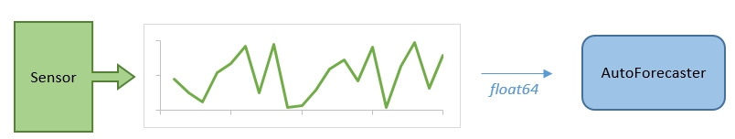
To analyze a single time series, each tuple consumed by the operator must contain an attribute of type float64, which represents a single point in the time series. For example, the following diagram shows a single sensor that periodically records a value and sends it to the AutoForecaster2. Each time the sensor records a value, a single data point is sent to the AutoForecaster2.

Here is an SPL snippet that demonstrates the operator analyzing a single time series:

(stream<float64 inputData> NetloadData) as NetloadSource = FileSource()
{
    param
        file : "netload.out" ;
}

(stream<float64 inputData, uint64 forecastedTimestamp, 
float64 forecastedResult>
    ForecastedResults) as ForecastingOperator = AutoForecaster2(NetloadTimeData)
{
    param
        inputTimeSeries : inputData ;
        initSamples : 100u ;
        stepAhead : 20u ;
        algorithm : Dynamic ;
    output
        ForecastedResults :
forecastedResult = forecastedTimeSeriesStep(,
            forecastedTimestamp = forecastedTimestamp() ;
}

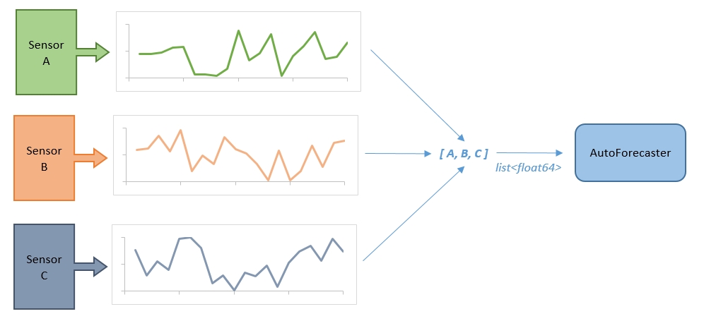
To analyze multiple, independent time series, each tuple consumed by the operator must contain an attribute of type list<float64>. Each element in the list contains a data point from each of the sensors at a single point in time. For example, the following diagram shows 3 independent sensors that periodically record values. At a given point in time, each sensor will record a value. Each of those recorded values, at the given point in time, will be added to a list. The list is then sent to the AutoForecaster2 operator, which will forecast a future value for each of the 3 sensors.

Here is an SPL snippet showing the operator analyzing multiple time series:

(stream<
list<float64> listInputData> NetloadData) as NetloadSource = FileSource()
{
    param
        file : "multi_netload.out" ;
}

(stream<list<float64> listInputData, uint64 forecastedTimestamp, 
list<float64> forecastedResult
>
    ForecastedResults) as ForecastingOperator = AutoForecaster2(NetloadTimeData)
{
    param
        inputTimeSeries : listInputData ;
        initSamples : 100u ;
        stepAhead : 20u ;
        algorithm : Dynamic ;
    output
        ForecastedResults :forecastedResult = forecastedTimeSeriesStep(),
            forecastedTimestamp = forecastedTimestamp() ;
}

Results

The AutoForecaster2 operator is not only capable of forecasting the next value in the time series, but can actually forecast several steps into the future. The number of future values (steps) that the AutoForecaster2 forecasts is controlled by the stepAhead parameter. When submitting results, the operator can output all of the values up to the specified number of steps.

There are two output functions used to return forecasted values:

forecastedTimeSeriesStep() – returns the forecasted time series value at step n, where n is the same as the stepAhead parameter value.
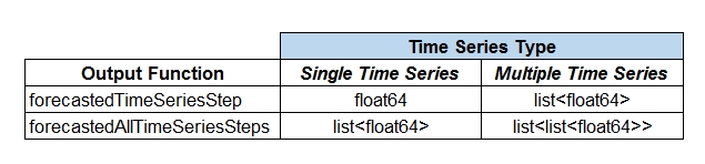
forecastedAllTimeSeriesSteps() – returns a list of forecasted time series values from step 1 to step n, where n is the same as the stepAhead parameter value.

Note: the return type of these output functions depends on whether the operator is analyzing a single time series or multiple time series. The following table shows the return type of these output functions based on the type of input data.

Timestamps

The operator is also capable of calculating the future timestamp values along with the forecasted values. In order to calculate the future timstamp values, the incoming data must contain an attribute of either timestamp or uint64. This inputTimestamp parameter value must refer to this attribute.

The operator contains two output functions used to return the calculated future timestamp values:

forecastedTimestampStep() – returns the calculated future timestamp value at step n, where n is the same as the stepAhead parameter value.
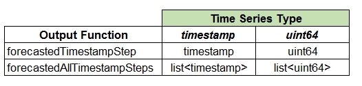
forecastedAllTimestampSteps() – returns a list of calculated future timestamp values from step 1 to step n, where n is the same as the stepAhead parameter value.

Note: the return type of these output functions depends on the type of the incoming timestamp attribute. The following table shows the return type of these output functions based on the type of the incoming attribute:

Parameters

The AutoForecaster2 operator comes with a number of parameters. Information regarding all of the available parameters can be found on the AutoForecaster2 Knowledge Center page. However, here are some of the important parameters:

inputTimeSeries – This parameter specifies the attribute on the input port that contains the time series data. The specified attribute must have a type of either float64 or list<float64>. This is a required parameter.

inputTimestamp – This parameter specifies the attribute on the input port that contains the timestamp information. While this parameter is optional, it must be specified in order to use the forecastedTimestampStep() and forecastedAllTimestampSteps() output functions.

initSamples – This parameter specifies the number of initial tuples that should be used to initially train the underlying algorithms. The number of samples to select depends on the type of data. For example, if the goal is to forecast results 1 day into the future, then this parameter should be set to a value that represents 1 day worth of data. It important to note that some of the underlying algorithms may use additional input data before initializing.

stepAhead – This parameter specifies how far into the future the operator should forecast. By default, this parameter is set to a value of 1.

algorithm – This parameter specifies whether the operator should continuously attempt to find a new algorithm (dynamic mode), or whether it should pick the best algorithm based on the initial set of training data and use that algorithm indefinitely (static mode). Since this topic if very important to the output of the operator, an entire section has been dedicated to explain the differences between dynamic and static mode.

Static vs Dynamic

In the introduction I mentioned that the AutoForecaster2 operator is capable of dynamically switching algorithms in order to produce the best possible forecasting. To be more specific, the operator comes with two modes: static mode and dynamic mode. Both of these modes will be discussed in detail below.

Static

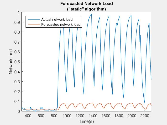
When the operator is set to static, it will use the initial set of input data to determine which algorithm provides the best forecasted results. Once the forecasting algorithm has been determined, that algorithm will be used for the remainder of the operator’s life. The advantage to running the operator in static mode is that it will be able to process tuples faster. This is due to the fact that the operator will only be forecasting future values and will not be continuously analyzing the incoming time series to find a better performing algorithm.

However, the disadvantage to using static over dynamic is that if the time series pattern changes dramatically over time, then the selected algorithm may no longer provide acceptable forecasted values. For example, assume the initial training data was mostly linear. In this case, it is likely that the AutoForecaster2 will select a linear regression algorithm to do the forecasting. Later on, if the time series data becomes non-linear, the forecasted values returned by the operator may not be accurate since a linear regression algorithm is unsuitable for this type of time series.

The following graph demonstrates this behavior. The blue line represents the actual network load that was captured and the orange line represents the forecasted values produced by the AutoForecaster2 operator. For the first 800 seconds, the network load is mostly flat (linear). However, after 800 seconds, the load begins to fluctuate dramatically. The operator was able to accurately forecast the load for the first 800 seconds, however once the time series pattern changed, the algorithm selected by the operator was no longer able to accurately forecast the values.

Dynamic

When the parameter value is set to dynamic, the AutoForecaster2 operator will continuously analyze the incoming time series values to determine the best forecasting algorithm. Each time a new tuple arrives, the operator will do the following:

1. Forecast the future time series values and submit the results to the operator’s output port (similar to static mode)
2. Analyze the current time series to determine if the current forecasting algorithm is still the best algorithm or if there is another algorithm that should be used (only done in dynamic mode)

These steps are repeated for every tuple that is sent to the AutoForecaster2. This allows the operator to adapt to changing time series patterns, thus enabling it to provide more accurate forecasted results. On the flip side, the consequence of setting the parameter value to dynamic is that the operator will spend more time processing a tuple (as compared to setting the value to static), ultimately decreasing the overall flow rate.

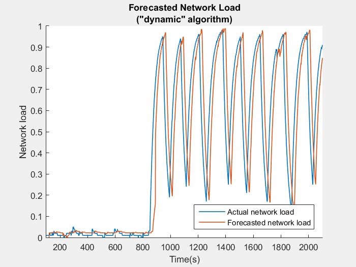
Revisiting the network load example above, we can clearly see the results of changing the algorithm parameter value to ‘dynamic’. Once again, the first 800 seconds are accurately predicted as being mostly linear in nature. However, when the input network load begins to fluctuate, the AutoForecaster2 is capable of automatically detecting this change and switching to a more accurate forecasting algorithm.

Conclusion

The AutoForecaster2 operator can be a powerful tool when building a Streaming application. It abstracts many of the complicated details of forecasting algorithms while still providing accurate and relevant results. The ability to dynamically switch algorithms at run-time is a key component of this operator and can be invaluable when analyzing unpredictable real-time data.

Samples

The network load example discussed early can be downloaded from GitHub here: https://github.com/IBMStreams/samples/tree/main/timeseries/AutoForecasterSamples.

Additional Links

AutoForecaster2 Operator – Knowledge Center

IBMStreams GitHub