This article was written by James Cancilla.

The DSPFilter operator implements a butterworth filter and can be used to isolate frequencies in a time series. For example, a low pass filter can be used to reject all frequencies above a certain point (this point is referred to as the cut-off frequency). Likewise, a high pass filter can be used to reject frequencies below a specific cut-off frequency.

While low pass and high pass filters are very useful, there are scenarios where you may need to isolate or reject frequencies within a certain range. These types of filters are called bandpass and bandstop filters.

A bandpass filter is used to isolate frequencies within a specific range. For example, you would use a bandpass filter if you wanted to isolate all frequencies between 100Hz and 200Hz, while filtering out all other frequencies.

A bandstop filter is the opposite of a bandpass filter. It allows for rejecting frequencies within a specific range, while allowing all other frequencies to pass. For example, a bandstop filter with cutoff frequencies of 400Hz and 600Hz would allow all frequencies below 400Hz and all frequencies above 600Hz to pass through the filter. Frequencies between 400Hz and 600Hz would be rejected.

Constructing the filters

In this exercise, we will construct a 2nd-order bandpass and bandstop filter using the DSPFilter operator. The exercise can downloaded from the IBMStreams/samples repository. Before we can begin constructing the SPL application, we first need to decide on the parameters for our filter. These parameters include the sampling rate and the cutoff frequencies.

The sampling rate (also referred to as the sampling frequency) is defined as the number of samples taken in one second. For this exercise, we will use a sampling rate of 2000Hz.

As mentioned previously, the cutoff frequencies define the range of frequencies that we either want to isolate or reject. For this exercise, we will use cutoff frequencies between 75Hz and 125Hz.

In summary, we have defined the following parameters:

Now that we have defined the parameters of our filter, we need to calculate the normalized cutoff frequencies. To do this, we simply divide each cutoff frequency by half the sampling rate.

Thus, our normalized cutoff frequencies are 0.075 and 0.125.

The equation to calculate a normalized frequency is: wn = f/(fs/2), where ‘wn’ is the normalized frequency being calculated, ‘f’ is the cutoff frequency and ‘fs’ is the sampling rate. Dividing the sampling rate by two (fs/2) produces the Nyquist frequency.

Now that we have the normalized frequencies, the next step is to determine the coefficients. For our filter. We will use R to calculate the coefficients, however other software such as Matlab© can also be used. R can be downloaded and installed from http://www.r-project.org/.

The R ‘signal’ library comes with a function called butter that is used to generate the filter coefficients. The butter function has the following definition:

We will only focus on the first 3 parameters. The first parameter, ‘n’ is used to specify the order of the filter. As mentioned previously, we will be constructing a second order filter, so this value will be 2. The second parameter, ‘W’, is used to specify the cutoff frequency (or frequencies). Finally, the ‘type’ parameter specifies the type of filter to generate the coefficients for.

We will begin by creating the bandpass filter. Enter the following into the R-console:

Entering ‘bf’ at the console will display the coefficients:

In the DSPFilter operator, there are 2 parameters that are used to specify the coefficients: xcoef and ycoef. The $b values from R are mapped to the xcoef parameter, and the $a values are mapped to the ycoef parameter.

Configure the DSPFilter

At this point, we have all of the information we need in order to configure the DSPFilter. It is simply a matter of plugging in the values and launching the test application.

The graph for the final application will look as follows.

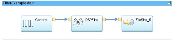
To configure the DSPFilter, there are only 3 parameters that we need to setup. When complete, the parameter list will look as follows.

inputTimeSeries : inputSignalAlias.signal ;

xcoef : { 0u : 0.005542717, 2u : - 0.011085434, 4u : 0.005542717 } ; 
ycoef : { 0u : 1.0000000, 1u : - 3.6048048, 2u : 5.0363144, 3u : -3.2247373, 4u : 0.8008026 } ; 

The first parameter is inputTimesSeries, which specifies the attribute on the input port that contains the signal data. The next two parameters are xcoef and ycoef, which we will populate with the coefficient values we calculated in R. The xcoef and ycoef parameters take values of type map<uint32, float64>. The map key (uint32) is the coefficient index and the map value (float64) is the corresponding coefficient value.

TIP: If the coefficient value is zero, you do not need to specify it in the map. The DSPFilter will automatically assume missing coefficient indexes to have a value of zero.

Finally, we need to set the DSPFilter’s output clause to output the filtered signal. The complete DSPFilter will look like this.

(stream<float64 origSignalValue, float64 filteredSignalValue>
    DSPFilter_4_out0) as DSPFilter_4 = DSPFilter(Generator_3_out0 as inputSignalAlias)
{
    param
        inputTimeSeries : inputSignalAlias.signal ;
        xcoef : { 0u : 0.005542717, 2u : - 0.011085434, 4u : 0.005542717 };
        ycoef : { 0u : 1.0000000, 1u : - 3.6048048, 2u : 5.0363144, 3u : -3.2247373, 4u : 0.8008026 } ;
    output
        DSPFilter_4_out0 : origSignalValue = inputSignalAlias.signal, 
        filteredSignalValue = filteredTimeSeries() ;
}

Testing the DSPFilter

To test this, we will connect a Generator operator to generate a sine wave at various frequencies.

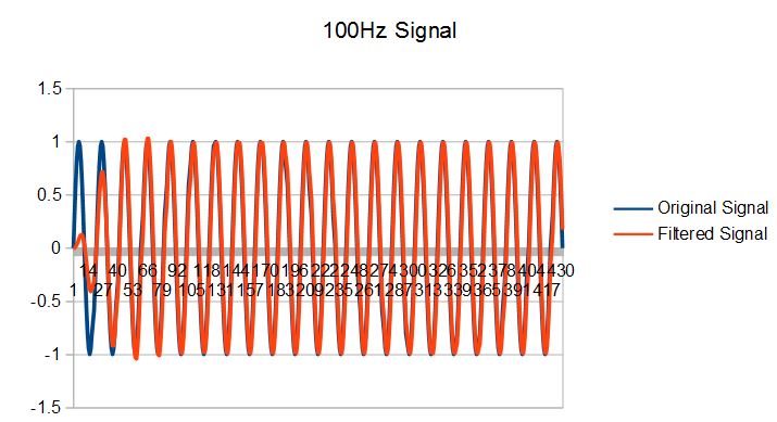
First, we will run the application by generating a 100Hz sine wave. Since our DSPFilter is configured to allow frequencies between 75Hz and 125Hz to pass through, we will not see any attenuation of the signal.

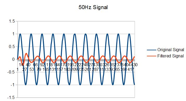
Next, we will generate a 50Hz and 200Hz sine waves. In both cases, we can see that the signals are significantly attenuated.

Bandstop filter

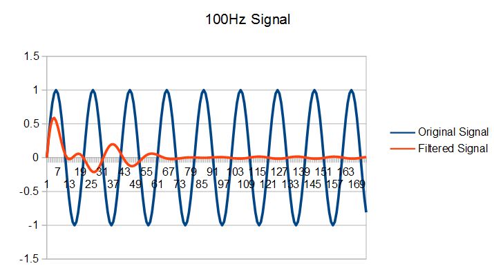
The bandstop filter is created the same way as described above. The only difference is that you need to set the ‘type’ argument for the butter function to ‘stop’ instead of ‘pass’. Doing so will generate a new set of coefficients specific to the bandstop filter. Here are some examples of using the bandstop filter with the same cut-off frequencies as before. Note that in this case, the 100Hz sine wave is significantly attentuated but the 50Hz sine wave has no attenuation.

Here is the SPL code for the DSPFilter implementing a ‘bandstop’ filter.

(stream<float64 origSignalValue, float64 filteredSignalValue>
        DSPFilter_4_out0) as DSPFilter_4 = DSPFilter(Generator_3_out0 as inputSignalAlias)
{
    param
        inputTimeSeries : inputSignalAlias.signal ;
        xcoef : { 0u : 0.8948586, 1u : -3.4147710, 2u : 5.0473998, 3u : -3.4147710, 4u : 0.8948586 } ;
        ycoef : { 0u : 1.0000000, 1u : -3.6048048, 2u : 5.0363144, 3u : -3.2247373, 4u : 0.8008026} ;
    output
        DSPFilter_4_out0 : origSignalValue = inputSignalAlias.signal, 
            filteredSignalValue = filteredTimeSeries() ;
}

Click here to download this example.

References:

http://www.mathworks.com/help/signal/ref/butter.html
http://cran.r-project.org/web/packages/signal/signal.pdf