Global AI and Data Science

Global AI & Data Science

Train, tune and distribute models with generative AI and machine learning capabilities

 View Only
  • 1.  Citi Bike 2017 Analysis

    Posted Sun May 06, 2018 11:42 AM

    Citi Bike 2017 Analysis 

    The goal of this analysis is to create an operating report of Citi Bike for the year of 2017. This is a fictional case based on real data. 

    Client: Mayor of New York City, Bill de Blasio
    Objective: Help the mayor get a better understanding of Citi Bike ridership by creating an operating report for 2017 (NYC only).

    Ask:

    1. Top 5 stations with the most starts (showing # of starts)
    2.  Trip duration by user type
    3. Most popular trips (based on start station and stop station)
    4. Rider performance by Gender and Age based on avg. trip distance (station to station), median speed (trip duration / distance traveled)
    5. What is the busiest bike in NYC in 2017? How many times was it used? How many minutes was it in use?
    6. A model that can predict how long a trip will take given a starting point and destination (Do not use the Google Maps API).

    The data was sourced from the Citi Bike's amazon server which can be accessed here. The code used for this article can be found here.*

    First, let's minimize the work and load in the data set. From the server, it's clear that these files are massive, a few hundred MBs each. 

    !curl -O "https://s3.amazonaws.com/tripdata/2017[01-12]-citibike-tripdata.csv.zip"
    !unzip '*.zip'
    !rm *.zip
    files = !ls *.csv #For Ipython only
    df = concat([read_csv(f, header=None,low_memory=False) for f in files], keys=files)

    The column names have spaces in them, would be great to remove them for working purposes. If I was working on a team or a long term project, I would configure column names a little bit differently to make them easier to work with. However, I've kept the names simple and easy to understand for the purposes of this article. 

    The dataset is massive, ~16mil rows. BigData tools would be helpful, however, most require you to pay or have an enterprise license or a limited trial. Additionally, the data is very dirty. Different files have different column names, need to account for this. Mayor de Blasio doesn't have a technical background. The graphs here are as simple yet informative as possible. I could've made more complicated plots, however, they would not be as informative for the mayor. The graphs are designed with the user in mind.

    Lastly, my analysis tries best to follow the crisp-dm methodology outlined below.

    Taken from researchgate.net

    Let's understand the data we're working with and give a brief overview of what each feature represents or should represent. 

    1. Trip Duration (seconds) - How long a trip lasted
    2. Start Time and Date - Self explanatory
    3. Stop Time and Date - Self explanatory
    4. Start Station Name - Self explanatory
    5. End Station Name - Self explanatory
    6. Station ID - Unique identifier for each station
    7. Station Lat/Long - Coordinates
    8. Bike ID - unique identifier for each bike
    9. User Type (Customer = 24-hour pass or 3-day pass user; Subscriber = Annual Member) - Customers are usually tourists, subscribers are usually NYC residents
    10. Gender (Zero=unknown; 1=male; 2=female) - Usually unknown for customers since they often sign up at a kiosk
    11. Year of Birth - Self entered, not validated by an ID.

    Part 1: Top 5 Stations

    Let's check if there's any noise or cleanup which needs to be done before creating the chart.

    1. Any missing values?
    • Mostly for Birth year
    •  Few for User Type.
    • Citi Bike customers (1-day pass or 3-day pass) are often tourists and may not put in their birth year in a rush or due to other reasons
    • Citi Bike subscribers tend to be NYC residents, by blindly dropping rows with missing values, we'll be losing critical information and may introduce bias.

    2. Let's get a description of the data we're working with:


    3. Citi Bike riders often come across broken bikes. As a user, I am quite familiar with the dilemma. Let's drop any trips where a trip lasted less than 90 seconds and the start station == end station. 90 seconds is an arbitrary choice based on how long it would take a rider to realize a bike isn't working properly and coming back to the station to return it and take a new on. Another measure which can be used is 372 seconds (25% quartile). This is based on the assumption that if someone is making a round trip, it most likely is to perform some quick task which is not close enough to walk to, thus this trip should be at least a little bit longer than the shortest trip.In case it was a short trip, let's add the extra and condition to make sure the start and end station names are the same. 

    4. Anomalies such as theft and broken docks shouldn't matter for this metric and can be dealt with later.

    Considered a pie chart for this, however, these stations make up less than 5% of the total starts in this dataset

    Part 2: Trip Duration by User Type

    This question is a bit unclear in terms of what to do with the anomalies, so I'll be making two graphs. One with anomalies, one without.

    There are NA values in the dataset for usertype as can be seen from missing table image above. Since it's only 0.09% of the data, it can be considered safe to remove.

    According to Citi Bikes' website: The first 45 minutes of each ride is included for Annual Members, and the first 30 minutes of each ride is included for Day Pass users. If you want to keep a bike out for longer, it's only an extra $4 for each additional 15 minutes.

    It's safe to assume, no one (or very few people) will be willing to rent a bike for more than 2 hours, especially a clunky citibike. If they did, it would cost them an additional $20 assuming they're annual subscribers. It would be more economical for them to buy a bike if they want that workout or use one of the tour bikes in central park if they want to tour and explore the city on a bike. There may be a better way to choose an optimal cutoff, however, time is key in a client project. Or just docing and getting another bike. The real cost of a bike is accrued ~24 hours.

    Anomalies: Any trip which lasts longer than 2 hours (7,200 seconds) probably indicates a stolen bike, an anomaly, or incorrect docking of the bike. As an avid Citi Bike user, I know first hand that it doesn't make any sense for one to use a bike for more than one hour! However, I've added a one hour cushion just in case. No rider would plan to go over the maximum 45 minutes allowed. However, I plan to reduce this to one hour in the future for modeling purposes.

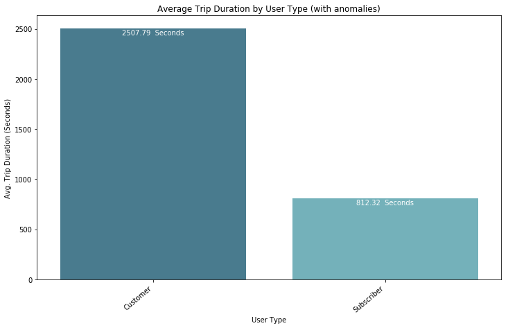
    1. First Half- with anomalies in dataset
    • The bargraph of average trip duration for each user type. It's helpful, but would be better to see a box-plot or violin plot. Would be easier to interpret in minutes.
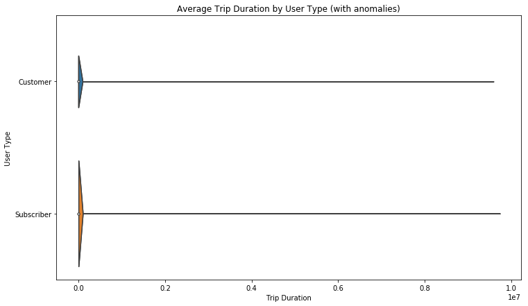
    • Second graph is a basic violin plot based with anomalies included. As we can see, there is too much noise for this to be useful. It'll be better to look at this without anomalies.

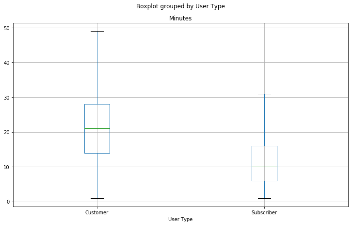
    2. Second Half - without anomalies in dataset

    • A much more informative graph about trip duration based on user type with anomalies defined as mentioned above. "Fliers" have been removed from the graph below.
    Note: User Type will most likely be a strong predictor of trip duration
    • Bar-graph highlighting average duration of each trip based on user type

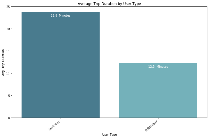
    It's safe to say that user type will be a strong predictor of trip duration. It's a point to note for now and we can come back to this later on. 


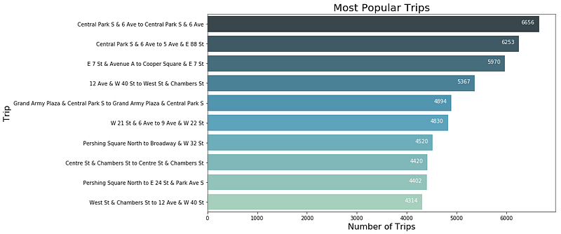
    Part 3: Most Popular Trip

    To get most popular trips, the most convenient way to do this is by using the groupby function in pandas. It's analogous to a Pivot table.

    trips_df = df.groupby(['Start Station Name','End Station Name']).size().reset_index(name = 'Number of Trips')

    The groupby function makes it extremely easy and convenient to identify the most popular trips. 


    Part 4: Rider Performance by Gender and Age

    Ask: Rider performance by Gender and Age based on avg trip distance (station to station), median speed (trip duration/distance traveled)

    Let's make sure the data we're working with here is clean.

    1. Missing Gender and Birth Year values? - Check missing_table above
    • No for Gender. Yes for Birth Year
    • ~10% Missing Birth year. Not a big chunk of data. Can either impute missing values or drop it. Since it's less than 10% of the data, it's safe to assume the rest of the 90% is a representative sample of data and we can replace the birth year with the median, based on gender and Start Station ID. I chose this method because most people the same age live in similar neighborhoods (i.e: young people in east village, older people in Upper East Side, etc.). This will be done after anomalies are removed and speed is calculated. There may be better ways to impute this data, please share your thoughts in the comments section below. 
    df['Birth Year'] = df.groupby(['Gender','Start Station ID'])['Birth Year'].transform(lambda x: x.fillna(x.median()))

    2. Are there anomalies?

    • For Birth Year, there are some people born prior to 1960. I can believe some 60 year olds can ride a bike and that's a stretch, however, anyone "born" prior to that riding a Citi Bike is an anomaly and false data. There could be a few senior citizens riding a bike, but probably not likely.
    • My approach is to identify the age 2 standard deviations lower than the mean. After calculating this number, mean - 2stdev, I removed the tail end of the data, birth year prior to 1956.
    df = df.drop(df.index[(df['Birth Year'] < df['Birth Year'].mean()-(2*df['Birth Year'].std()))])

    3. Calculate an Age column to make visuals easier to interpret:

    df['Age'] = 2018 - df['Birth Year'];
    df['Age'] = df['Age'].astype(int);

    4. Calculate trip distance (Miles)

    • No reliable way to calculate bike route since we can't know what route a rider took without GPS data from each bike.
    • Could use Google maps and use lat, long coordinates to find bike route distance. However, this would require more than the daily limit on API calls. Use the geopy.distance package which uses Vincenty distance uses more accurate ellipsoidal models. This is more accurate than Haversine formula, but doesn't matter much for our purposes since the curvature of the earth has a negligible effect on the distance for bike trips in NYC.
    • In the future, for a dataset of this size, I would consider using the Haversine formula to calculate distance if it's faster. The code below takes too long to run on a dataset of this size.
    dist = []
    for i in range(len(df)):
    dist.append(geopy.distance.vincenty(df.iloc[i]['Start Coordinates'],df.iloc[i]['End Coordinates']).miles)
    if (i%1000000==0):
    print(i)

    5. Calculate Speed (min/mile) and (mile/hr)

    • (min/mile): Can be used like sprint time (how fast does this person run)
    df['min_mile'] = round(df['Minutes']/df['Distance'], 2)
    • (mile/hr): Conventional approach. Miles/hour is an easy to understand unit of measure and one most people are used to seeing. So the visual will be created based on this understanding.
    df['mile_hour'] = round(df['Distance']/(df['Minutes']/60),2)

    6. Dealing with "circular" trips

    • Circular trips are trips which start and end at the same station. The distance for these trips will come out to 0, however, that is not the case. These points will skew the data and visuals. Will be removing them to account for this issue.
    • For the model, this data is also irrelevant. Because if someone is going on a circular trip, the only person who knows how long the trip is going to take is the rider, assuming s/he knows that. So it's safe to drop this data for the model.
    df = df.drop(df.index[(df['Distance'] == 0)])

    7. We have some Start Coordinates as (0.0,0.0). These are trips which were taken away for repair or for other purposes. These should be dropped. If kept, the distance for these trips is 5,389 miles. For this reason I've dropped any points where the distance is outrageously large. Additionally, we have some missing values. Since it's a tiny portion, let's replace missing values based on Gender and start location. 

    Apologies for separate images
    • On some trips, the speed of the biker is more than 200 mph. This could be due to the formula used for distance calculation or some other error. The fastest cyclist in the world on a flat surface ever recorded biked at 82mph. It's safe to assume none of the Citi Bike riders can approach this speed. Due to this and the fact that an average cyclist speed is 10mph, I've decided to remove all data where the speed in mph is greater than 20 mph and less than 2 stdev from the mean, because that's probably a roundtrip where the biker found the dock was full and used another dock instead. 

    8. Rider performance by age and gender in miles/hour, after data cleaning

    There's a bit of a difference in speed, however, it doesn't seem drastic enough to have a major impact. Surprising thing is that age doesn't have a strong impact on speed either.

    9. Rider performance by age and gender in average distance in miles

    Barely a difference in distance travelled, age doesn't seem to have an impact either except for folks aged 16–25


    Part 5: Busiest Bike by Times and Minutes Used

    Ask:

    1. What is the busiest bike in NYC in 2017?
    2. How many times was it used?
    3. How many minutes was it in use?
    • Busiest bike and count can be identified by a group-by function. Function below will also identify the number of times the bike was used
    bike_use_df = df.groupby(['Bike ID']).size().reset_index(name = 'Number of Times Used');
    bike_use_df = bike_use_df.sort_values('Number of Times Used', ascending = False);
    Most popular bike by number of times used: Bike 25738 (2355 times)
    • A similar groupby function which calls for the sum on minutes can identify the number of minutes the bike was used.
    bike_min_df['Minutes Used'] = df.groupby('Bike ID')['Minutes'].sum()
    bike_min_df = bike_min_df.sort_values('Minutes Used', ascending = False)
    Most popular bike by number of minutes used: Bike 25738 (31,340 minutes)

    Part 6.1: Predictive Model - Baseline Model

    Ask: Build a model that can predict how long a trip will take given a starting point and destination.

    Assumptions on how the Kiosk will work: Let's assume that when a user inputs the start and end station, they swipe their key fob (if they're a subscriber) and enter their info on the kiosk (if they're a "Customer") prior to entering the start and end station. This means that we would know their gender and age. Thus these variables can be used in building the model.

    Step 1.

    • This dataset is massive. Almost 14 million rows. Let's work on a random subsample while we build and evaluate models. If I tried to build and evaluate a model on the entire dataset, each run would take me ~10+ minutes depending on the model. One good way to decide what portion of your data to work with is using a learning curve. However, my kernel keeps crashing while trying to create that learning curve. If we were working with data for multiple years, we would need to reconsider this approach. However, given the reasons above, let's sample 10% of the data. It's still ~1.3 million rows and should be a representative sample since it's randomly selected. To ensure that it's a representative sample, we should look at the description of the original dataset and the sample dataset. Lastly, we can make sure the data is representative by making the the visuals above are the similar for the random sample. 10% of the data passes the test above.
    • Additionally, Citi Bike trips are capped at 45 minutes for subscribers and 30 minutes for customers (refer to "According to Citi Bike's website" above). After these respective time limits, the riders incur a fee. To model our data, it does not make sense to include trips which last longer than the prescribed 45 minutes. Rider's don't often plan to go over the allocated time and there's no clear way of knowing who plans to go over the allocated time. It's a question worth exploring, however, the data is noise for our model. 
    df = df.drop(df.index[(df['Trip Duration'] > 2700)])
    df_sample = df.sample(frac = 0.1, random_state = 0)

    Step 2.

    • Let's get a baseline. If I were to just run a simple multi-variate linear regression, what would my model look like and how accurate would it be? Need to prepare the data for a multivariate regression
    1. Drop irrelevant columns
    • Trip Duration: We have the minutes column, which is the target variable
    • Stop Time: In the real world, we won't have this information when predicting the trip duration.
    • Start Station ID: Start Station Name captures this information
    • Start Station Latitude: Start Station Name captures this information
    • Start Station Longitude: Start Station Name captures this information
    • Start Coordinates: Start Station Name captures this information
    • End Station ID: End Station Name captures this information
    • End Station Latitude: End Station Name captures this information
    • End Station Longitude: End Station Name captures this information
    • End Coordinates: End Station Name captures this information
    • Bike Id: We won't know what bike the user is going to end up using
    • Birth Year: Age captures this information
    • min_mile: Effectively the same information as end time when combined with distance. We won't have this information in the real world.
    • mile_hour: Effectively the same information as end time when combined with distance. We won't have this information in the real world.
    (Speed * Distance = Trip Duration): Which is why speed is dropped
    • Start Station Name and End Station Name: The distance variable captures the same information. For the model, if a user is inputting start and end station, we can build a simple function to calculate the distance which would capture the same information. One may argue to keep this information since this is the information which will be provided at the kiosk. However, given that there are over 800 stations, if we keep this information, we are required to encode this for any regression algorithm. This would create 800 features (~15 million rows) leading to lots of data, without much, if any, information gain. 
    After the cleaning mentioned above, the final predictors used for the baseline model are Distance, User Type, and Gender. Age seems to have no impact as can be seen by the visuals in part 4. To confirm this, I ran the model with and without age. Age had little to no impact on the model. 

    • I chose to run a linear regression. The size of the data and limitation of resources made running more complex models less attractive. Ensemble algorithms were tested, but took too long to run.
    • The model is pretty good for a baseline model with an R² and Adjusted R² of 0.774. Distance seems to be having a large impact on trip duration, which makes sense. 


    Part 6.2: Predictive Model - Including Date

    Steps to make improvements: 

    1. Add back time in the following format

    • Is the ride on a weekday or weekend. Weekday, is rush-hour commute for the most part and probably from home to work. Weekend could be a longer, more casual ride and have higher variability.
    • Is the ride in the morning, afternoon, evening, or night. The exact timing will be based on the difference in trip duration based on time of day. Will have visuals below.

    2. What season is it?

    • December - Feb. = Winter
    • March - May = Spring
    • June - Aug. = Summer
    • Sept. - Nov. = Fall
    def get_date_info(df):
    df['d_week'] = df['Start Time'].dt.dayofweek
    df['m_yr'] = df['Start Time'].dt.month
    df['ToD'] = df['Start Time'].dt.hour

    df['d_week'] = (df['d_week']<5).astype(int)

    df['m_yr'] = df['m_yr'].replace(to_replace=[12,1,2], value = 0)
    df['m_yr'] = df['m_yr'].replace(to_replace=[3,4,5], value = 1)
    df['m_yr'] = df['m_yr'].replace(to_replace=[6,7,8], value = 2)
    df['m_yr'] = df['m_yr'].replace(to_replace=[9,10,11], value = 3)

    df['ToD'] = pd.cut(df['ToD'], bins=[-1, 5, 9, 14, 20, 25], labels=['Night','Morning','Afternoon','Evening','Night1'])
    df['ToD'] = df['ToD'].replace(to_replace='Night1', value = 'Night')
    df['ToD'] = df['ToD'].cat.remove_unused_categories()

    df['m_yr'] = df['m_yr'].astype('category')
    df['d_week'] = df['d_week'].astype('category')

    return(df)
    • Model 1: Negligible improvement in R²: 77.7% (depending on random_state used)
    • Safe to assume that we can drop these variables as they don't have a major impact. 
    • It's a bit surprising that the weekday variable has little to no impact since people most likely bike for leisure on weekends rather than for work. This could be explained by obtaining a breakdown of riders. Maybe a lot of Citi Bike users are college students. 
    • Another possibility is that the effect of this feature is being skewed by the fact that there are both customers and subscribers in this dataset and the effect of this feature on both variables is different. However, there's no clear explanation for now. It's worth considering building a separate model for subscribers and customers since their behavior is so drastically different as seen in part 2.

    Part 6.3: Predictive Model - Improving Model 1

    • Next steps will be to factor in speed and distance based on Gender and Trip. By not being able to encode start and end stations (due to the sheer number of points), we are losing crucial information on the trip itself. We need another proxy for those measures.
    • Another change I could make is to bin age into buckets. However, the data indicates that age has no correlation or effect on the trip duration. This is counter-intuitive, however, I don't have a good reason to refute the data.
    1. Include Average Speed based on: Trip (Start + End Station) and User Type. 
      1. Reason for Trip: Some trips are up hill, others are down hill. Some routes, such as one through times square involve heavy traffic, based on intuition.
      2. Reason for User Type: Tourists (Customers), will usually ride more slowly with frequent stops than a Subscriber, according to the data.

    2. Include average duration for each trip based on: Trip and User Type for reasons mentioned above

    def get_speed_distance(df):

    df['Start Station Name'] = df['Start Station Name'].astype(str)
    df['End Station Name'] = df['End Station Name'].astype(str)
    df['Trip'] = df['Start Station Name'] + ' to ' + df['End Station Name']
    df['Trip'] = df['Trip'].astype('category')

    df['avg_speed'] = df.groupby(['Trip','User Type'])['mile_hour'].transform('mean')
    df['avg_duration'] = df.groupby(['Trip','User Type'])['Trip Duration'].transform('median')

    return df
    • The model is significantly better. But can it be even better?
    • One factor which would have a significant impact on trip duration is traffic. However, since we do not know what route the rider took it's difficult to incorporate this information. Lastly, the Google Maps API caps usage, so we can't use it to identify traffic patterns easily.

    Part 6.4: Predictive Model - Improving Model 2

    • One factor which a lot of people think may be a good predictor of trip duration is weather. I personally disagree. Weather influences wether or not a user will bike, not how long they will bike. If it's snowing, I won't bike to work. If it's nice, I will bike to work. Regardless of my opinion, I am going to test this hypothesis. If weather is not a strong indicator, I will remove it in the next model.
    • The weather data was acquired from the National Centers for Environmental Information. The data sourced from the website is a daily summary. The attributes include: high temperature (F), low temperature (F), and precipitation (inches).
    def get_weather(df):
    df['DATE'] = to_datetime(df['Start Time'].dt.date)
    df = df.merge(df_weather, on = 'DATE', how = 'left')
    return df
    • Little to no improvement in the model. Weather has little to no impact. 
    • The coefficient for avg_duration spiked up. Not sure why, but the higher coefficient makes sense since duration is our target variable, and avg_duration is a solid proxy (anchor) for how long a trip most likely takes. 
    • Let's confirm the effectiveness of the model with cross validation:
    CV accuracy: 0.874 +/- 0.001
    • Based on some of the observations above I ran the same model above without weather and date information as predictors.  
    • As we can see, there's a very small decrease in R². Another interesting observation is the effect of this data on the coefficient of user type, it's almost halved.
    • The effect on the random sample is small, however, with 10 times the amount of data, the effect could be slightly larger, so for the final model, let's keep the date information.
    • Lastly, I chose to test other regression algorithms such as random forests to see if another regressor performed better. I chose to keep the n_estimators low due to run-time concerns. With this parameter set to 80, the model took 10 minutes to run with an R² the same as that of the linear regression. It could be worth pursuing random forests by optimizing other parameters such a min_samples_leaf. One approach may be to see the distribution of trip duration to identify the number of of trips which take 5–6 minutes, 6–7 minutes, etc. This could help identify the min_samples_leaf parameter. In the real world, we don't need to be accurate to the exact second. As long as we can predict how long the trip will take within a minute, it's a solid result in my opinion. Google maps doesn't tell you how long your trip will take to the exact second, it gives you it's prediction as an integer in minutes. 

    Part 6.5: Predictive Model - Final Model

    • I could've used XGboost and other fancy algorithms, however, for a dataset of this size, it would take too long to run and the gains wouldn't be worth it if there are any.
    • Final Model: Linear Regression (worth exploring Lasso)
      • Predictors: Distance, Gender, Average Duration and Average Speed based on Trip and Gender, User Type, and Date information
    CV accuracy: 0.852 +/- 0.000


    *The code is a work in progress and constantly undergoing changes and improvement with your feedback. Please leave your thoughts in the comments section below. Thank you.


    ------------------------------
    Vinit Shah
    ------------------------------

    #GlobalAIandDataScience
    #GlobalDataScience


  • 2.  RE: Citi Bike 2017 Analysis

    Posted Mon May 07, 2018 06:10 AM
    Interesting. Thanks for sharing.

    ------------------------------
    Surendra Goud E V Goud E V
    ------------------------------