Time series is a series of data points indexed (or graphed) in time sequence, for example, daily stock prices or weekly sales data. Commonly, a time series is a sequence that is taken at successive equal intervals of any time unit, such as second, hour or day, week, so it is a sequence of discrete-time data.
Time series example: IBM stock price of past 5 years from 2014 to 2018

Characteristics of Time Series
Time series data have a natural temporal ordering. This makes it different from data that there is no natural ordering of the observations (like explaining people's wages by reference to their respective education levels, where the individuals' data might be entered in any order).
Time series analysis is also distinct from spatial data analysis where the observations typically relate to geographical locations (for example, accounting for house prices by the location as well as the intrinsic characteristics of the houses). Time series data is frequently plotted via line charts, when plotted, most time series exhibit one or more of the following features:
A trend is a gradual upward or downward shift in the level of the series or the tendency of the series values to increase or decrease over time.
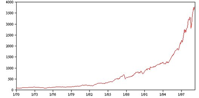
Trends are either local or global, but a single series can exhibit both types. Historically, series plots of the stock market index show an upward global trend. Local downward trends have appeared in times of recession, and local upward trends have appeared in times of prosperity.
- Seasonal and nonseasonal cycles
A seasonal cycle is a repetitive, predictable pattern in the series values.
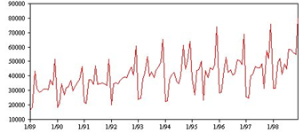
Seasonal cycles are tied to the interval of your series. For instance, monthly data typically cycles over quarters and years. A monthly series might show a significant quarterly cycle with a low in the first quarter or a yearly cycle with a peak every December. Series that show a seasonal cycle are said to exhibit seasonality.
Seasonal patterns are useful in obtaining good fits and forecasts, and there are exponential smoothing and ARIMA models that capture seasonality.
A nonseasonal cycle is a repetitive, possibly unpredictable, pattern in the series values.
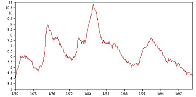
Some series, such as unemployment rate, clearly display cyclical behavior; however, the periodicity of the cycle varies over time, making it difficult to predict when a high or low will occur.
Nonseasonal cyclical patterns are difficult to model and generally increase uncertainty in forecasting.
Many series experience unexpected changes in level. They generally come in two types:
- A sudden, temporary shift, or pulse, in the series level
- A sudden, permanent shift, or step, in the series level
When steps or pulses are observed, it is important to find a plausible explanation. Time series models are designed to account for gradual, not sudden change. As a result, they tend to underestimate pulses and be ruined by steps, which lead to poor model fits and uncertain forecasts. (Some instances of seasonality might appear to exhibit sudden changes in level, but the level is constant from one seasonal period to the next.)
Shifts in the level of a time series that cannot be explained are referred to as outliers. These observations are inconsistent with the remainder of the series and can dramatically influence the analysis and, consequently, affect the forecasting ability of the time series model.
In the following trend chart, outlier observation is marked with *
Outlier detection in time series involves determining the location, type, and magnitude of any outlier's present. Tsay (1988) proposed an iterative procedure for detecting mean level change to identify deterministic outliers. This process involves comparing a time series model that assumes no outliers are present to another model that incorporates outliers. Differences between the models yield estimates of the effect of treating any given point as an outlier.
- Autocorrelation function (ACF) and Partial autocorrelation function (PACF)
Autocorrelation and partial autocorrelation are measures of association between current and past series values. They indicate which past series values are most useful in predicting future values. With this knowledge, you can determine the order of processes in an ARIMA model.
Autocorrelation function (ACF). At lag k, this is the correlation between series values that are k intervals apart.
Partial autocorrelation function (PACF). At lag k, this is the correlation between series values that are k intervals apart, accounting for the values of the intervals between.
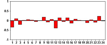
The x axis of the ACF plot indicates the lag at which the auto correlation is computed; the y axis indicates the value of the correlation (between −1 and 1). For example, a spike at lag 1 in an ACF plot indicates a strong correlation between each series value and the preceding value, a spike at lag 2 indicates a strong correlation between each value and the value occurring two points previously.
- A positive correlation indicates that large current values correspond with large values at the specified lag; a negative correlation indicates that large current values correspond with small values at the specified lag.
- The absolute value of a correlation is a measure of the strength of the association, with larger absolute values indicating stronger relationships.
Time Series Exploration(TSE)
TSE initially analyzing the characteristics of time series data based on basic statistics and tests. Useful insights are generated about the data before building the time series forecast model. TSE contains the following methods:
- TSE has several different algorithms for exploring the underlying behavior of time series.
- For single (univariate) time series, like temperature records of a day, TSE can:
- Use automatic exploration to decompose the series into a trend-cycle, seasonal, and irregular components to test for the following:
- Trend
- Turning points in trend
- Seasonality
- Outliers
- Level Shift, the level of time series suddenly changes to the other level.
- Variance change
- Unexplained autocorrelation
- Test for unit roots to determine whether the series is stationary (there is no trend in the time series).
- Use autocorrelation (ACF) and partial autocorrelation (PACF) to detect if past values of the series are correlated with present values.
- For pairs of (bivariate) time series, such as the height and weight of a child, TSE can:
- Use cross-correlation (CCF) to detect if past values of one series are correlated with present values of the other series.
- For a large number of series, such as daily water consumption data of one year, for all 3400 families in one area, TSE also offers two-step clustering to group time series that have similar time series-specific features.
Australian Relative Wool Prices Use Case
Each week that the market is open the Australian Wool Corporation sets a floor price that determines their policy on intervention and is therefore a reflection of the overall price of wool for the week in question. Actual prices that are paid can vary considerably from the floor price.
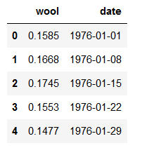
The data that is collected for the wool has two columns: weekly data log of the ratio between the price for fine grade wool and the floor price (wool) and the date variable (date). The time series are over a period of 309 weeks from 1976 through 1986. In this use case, we will explore the wool time series by applying the automatic time series exploration. The data set can download from package “boot” in R.
autowool.csv
Because TSE is meant to find time series data characteristics, and the insight of wool price, we use the SPSS TSE algorithm to explore this data on the IBM Watson Studio platform. Here the data has been imported as pandas data frame "df_data_1" and the first five lines display the following information:
 This notebook can be accessed by using this link
Notebook_TSE_UC1_autowool
To start the time series exploration
1. Convert data frame to sql context for the TSE algorithms process
from pyspark.sql import SQLContext
from pyspark.sql.types import *
from datetime import datetime
from pyspark.sql.functions import col, udf
from pyspark.sql.types import TimestampType

sqlCtx = SQLContext(sc)
df_sql = sqlCtx.createDataFrame(df_data_1)
func =  udf (lambda x: datetime.strptime(x, '%Y-%m-%d'), TimestampType())
df_sql = df_sql.withColumn('date1', func(col('date'))).drop("date").withColumnRenamed("date1", "date")
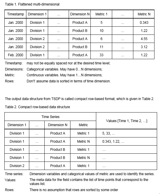
2. Build the TSE model by using the Auto Exploration feature. Note that the SPSS Time Series Data Preparation (TSDP) model is required before TSE. It converts the format of the raw data to the required format of the SPSS time series model.
TSDP is designed to coverts raw time series data (Flattened multi-dimensional, shown in Table 1) into regular data that SPSS TSE, TCM, and TSC components requiring (compact row-based, shown in Table 2).
from spss.ml.forecasting.timeseriesdatapreparation import TimeSeriesDataPreparation
from spss.ml.forecasting.timeseriesexploration import TimeSeriesExploration
from spss.ml.forecasting.reversetimeseriesdatapreparation import ReverseTimeSeriesDataPreparation
from spss.ml.common.wrapper import LocalContainerManager
lcm = LocalContainerManager()
tsdp = TimeSeriesDataPreparation(lcm). \
setMetricFieldList(["wool"]). \
setDateTimeField("date"). \
setEncodeSeriesID(False). \
setInputTimeInterval("WEEK"). \
setOutTimeInterval("WEEK"). \
setConstSeriesThreshold(0.0)
tsdpOutput=tsdp.transform(df_sql)
tse = TimeSeriesExploration(lcm). \
setInputContainerKeys([tsdp.uid]). \
setAutoExploration(True). \
setMaxACFLag(29)
tse_model=tse.fit(tsdpOutput)
tseOutput= tse_model.containerSeq()
statxml = tseOutput.entryStringContent("StatXML.xml")
json0 = tseOutput.entryStringContent("0.json")
print("0.json:\r\n"+json0)
0.json
From this example, we can see that the output of the SPSS TSE algorithm are json and statXML files, The json output includes all elements/values used for Trend/ACF/…. Plot, so user might need to integrate the output of TSE with the python matplotlib or the user application for TSE output visualization.
3. Get trend, irregular data, and turning points, outliers from json output, by using python matplotlib to plot sequence chart
jsonData=json.loads(json0)
y_trend=jsonData['univariate']['automaticExploration']['timeSeriesDecomposition']['trend_cycle']
y_irregular=jsonData['univariate']['automaticExploration']['timeSeriesDecomposition']['irregular']
index_turn_points=jsonData['univariate']['automaticExploration']['trendDetail']['turningPoints']
index_outlier=jsonData['univariate']['automaticExploration']['irregularDetail']['outlierDetection']['dateTime']
df_trend = df_data_1.copy()
df_irregular = df_data_1.copy()
df_trend.loc[:,'trend']=y_trend
df_trend.loc[index_turn_points,'turning_points']=df_trend.loc[index_turn_points,'trend']
df_trend.loc[index_outlier,'outlier']=df_trend.loc[index_outlier,'wool']
df_irregular.loc[:,'irregular'] = y_irregular
df_irregular.loc[index_outlier,'outlier']=df_irregular.loc[index_outlier,'irregular']
df_irregular.drop(['wool'], axis=1, inplace=True)
variation_interval=jsonData['irregularDetail']['variationAnalysis']['groupAnalysis']['interval']
variation_interval=[row[0] for row in variation_interval]
import matplotlib.pylab as plt
%matplotlib inline
from matplotlib.pylab import rcParams
import matplotlib.pylab as plt
%matplotlib inline
from matplotlib.pylab import rcParams
fig = plt.figure(figsize=(16,10))
styles1=['c.','','ro','rx']
styles2=['','rx']
ax1 = fig.add_subplot(211)
df_trend.plot(x='date', ax=ax1, title="trend", style=styles1)
ax2 = fig.add_subplot(212)
df_irregular.plot(x='date', ax=ax2, title="irregular", style=styles2)
for x in variation_interval:
plt.axvline(x,color='g')
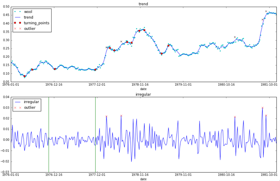
From TSE model and sequence charts, we can see
- In the TSE json output, time correlation of the wool series is 0.7858733; Trend-cycle component of wool series trended upwards, which shows overall that the wool price is increasing from 1976 through 1986.
- The direction of the trend-cycle component changes at week 16, 25, 51, 98, 115, 120, 135, 140, 149, 155, 175 and 183. The relative change and duration of change of each turning point are as follows
- Five outliers are detected in the irregular component series
- Wool prices can be aggregated to 3 groups with interval [0,43],[44,97],[98,308], by it's irregular variance. In 1977, the wool price is stable, but starting from year 1978, the wool price varies significantly.
4. Get Auto Correlation Function (ACF) chart
import numpy as np
lag=jsonData['univariate']['automaticExploration']['irregularDetail']['autoCorrelationAnalysis']['lag']
y_acf=jsonData['univariate']['automaticExploration']['irregularDetail']['autoCorrelationAnalysis']['acfValues']
y_ci=jsonData['univariate']['automaticExploration']['irregularDetail']['autoCorrelationAnalysis']['confidenceInterval']
plt.figure(figsize=(16,5))
x=np.arange(lag)
a=plt.bar(x,y_acf,color=(0.1, 0.1, 0.1, 0.1),label='Coefficient')
b=plt.plot(x,y_ci,label='Confidence Limit')
plt.ylabel("ACF")
plt.xlabel("Lag Number")
plt.title("Irregular")
plt.legend(loc='lower right')
plt.show()
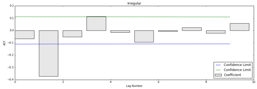
From the plot, we can see that the weekly data has a significant auto correlation. The wool price two weeks ago affects the wool price in the current week.
Summary:
1. Australian wool price shows an overall upward trend and the direction of price changes at given time points.
2. Five wool price outliers are detected, which need to be investigated further.
3. Wool prices have a significant correlation because, the price from two weeks ago affects the current week's wool price.
Locating IBM SPSS TSE
- IBM Watson Studio includes all the SPSS algorithms
- API documentation for Spark and Python is located here
#GlobalAIandDataScience#GlobalDataScience