Machine Learning : A methodology to train the machine to predict the future.
Basically Classified as:
Supervised Learning:
Classification , Regression classification:
binary Classification, where the target classes are two in number
multiclass Classification, where the target classes are more than two
Select the performance Measure:
RMSE

In binary case, the classes are often termed as positive or negative class that varies with the target variable to be predicted in a specific scenario.
In case to predict he spam: the target variable is negative
In Regression: The goal is to predict the target variable, which is contiunous / floating point number(Programming terms)/real number(Mathematical term)
Example:
To predict the salary of person
To predict the agricultural yield for a year
Generalization, Overfitting, underfitting:
Terms are particular to supervised learning:
In supervised learning, the Model is trained against the data set and the model is expected to predict the unseen data with the same characteristics the model is trained against, In model predicts well, means its able to generalization and more accurate the predicted better is the generalization by Model.
The Model might fell prey to following:
Overfitting, when the Model developed is too complex and that performs well on training data set as it’s fitting too closely with the particular characteristics of training date, hence can’t generalize on test data.
In other case, if the model being choosen is too simple, than the can’t perform well on training and test data
Solution: to fit the sweet spot( the Model complexity to be neither too simple nor too complex). As in KNN Algorithm, the value for k if too low or too high might drop the accuracy as for K too high , model become to simple( hence under fitting) and if K too low, than model turns too complex, hence Over fitting
The dataSet need not only use the measurements given in the input dataset as features but also using product of all features( called interactions) between the features , thus called feature Engineering.
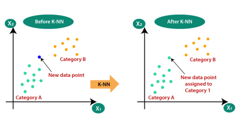
KNN : Classification
Model evaluation can be done using the score method: which for regression is R2 score( also called coefficient of determination), ranging between 0 to 1, 1 being perfect prediction.
Strength and weaknesses for KNN:
Number of neighbours and the distance measure , Euclidean or ?
KNN gets trained fast but performs poor with very large dataset or sparse dataset( where most of the features are zero)
Generally NOT used too aggresivley in real time
Impact of dataSet Size on Model Complexity:
Since model complexity is tied to the input variations hence, more is data set for training more Complex the model could be.
Un Supervised Learning: Pattern Detection
In the coming example we are going to use the following:
Python 3: being enriched in Machine learning APIs
SciPy: The Package for Python with
NumPy: The python library for the data structures
matplolib: For plotting the data
Sci-Kit Learn : The machine learning library
Linear Models
Used extensively. These models makes prediction using a linear function of the input features
y = m1*x1 + m2*x2 + m3*x3 +……………….+mn*xn +b
where x1 to xn are n input parameters and m and b are the parameters of Model that are learned and y is the prediction that Model makes.
Linear Models for regression differs on :
How model learns the parameters w and b
How the Model Complexity be controlled
Mostly used models are:
1. Linear Regression(ordinary least square)
2. Ridge Regression
3. Lasso
1. Linear Regression(ordinary least square)
This intend to find the values foe w and b that minimizes the mean squared error between predictions and the true regression targets y, on training dataset.
Since Linear Regression has no parameters, so easy to determine the mean squared error , but has NO way to control the Complexity.
The Slope parameters are called weights OR coofficients
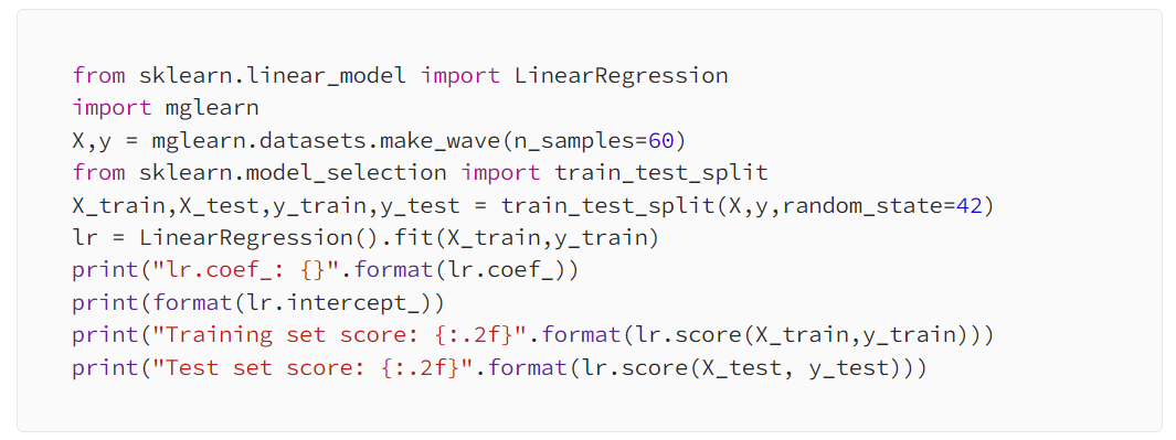
Possible suspect for Underfitting as the training score is also low and comparable to test score
Linear Models are less prone to underfitting for high dimensional dataSets but might fall prey to overfitting
In such scenario the high score for traing data and low score for test data signifies the high chances for Overfitting, and since the complexity cannot be controlled hence comes Ridge Regression for Rescue.
Ridge Regression:
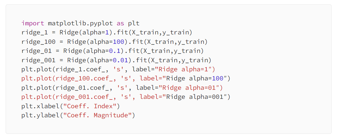
This Model in addition to the previous least square Model adds an additional constraint that enforces the magnitude of the coefficients to be as least as possible( intending them to be close to zero) that ensures the minimum effect of the coefficients on the outcome but still predicting well and is called regularization(L2 Regularization)
In case of Ridge regression,
training score will be less and the testing score will be high wrt Linear Regression(ordinary least square), since this will have less over fitting as its restricted and hence less complex Model so have poor performance on training data but better Generalization, hence,
Ridge implementation has:
Trade Off between the simplicity of Model( Non -Zero Coefficients ) and performance on training data Set. Alpha is parameter used to control the over fit.
More is Alpha , more forcefully coefficients made to reach near ZERO and hence tough training BUT more generalization
Also, lower the alpha means lower the restriction on coefficients and hence Ridge regression as good as Linear Regression
Alpha values can be altered:
Lasso: This is alternative to Ridge for the regularizing the linear regression. This also restricts the coefficients but to be close to zero, hence some coefficients are exactly zero, called L1 regularization, hence the automatic feature selection.it has regularization parameter called ALPHA, which controls how strongly coefficients are pushed towards zero.
import matplotlib.pyplot as plt
from sklearn.linear_model import Lasso
import numpy as np
lasso = Lasso().fit(X_train,y_train)
print(“Train set score :{}”.format(lasso.score(X_train,y_train)))
print(“Test set score :{}”.format(lasso.score(X_test,y_test)))
print(“Features used :{}”.format(np.sum(lasso.coef_ !=0)))
Usually Ridge Regression is first choice BUT in case we need the more explanatory model OR we have many parameters BUT only few are important, than Lasso will be preferred as it makes the feature selection by removing the irrelevant features itself.
Linear Model for Classification:
Most commonly used Algorithms are:
Logistic Regression
Linear SVM(Support Vector Machines)
Both these will have a trade Off factor called C , which is inversely related to regularization.
Higher the value C, lower the regularization , hence models try to fit data set as much as possible hence more likely to get over fit.
OR
low values for C, means high regularization, hence Model is stressed to classify each Data Point correctly and for high values of C, its like to adjust “majority” of data points
Linear Model for multiclass Classification:
A technique to extend the Binary Classification to multiclass Classification Algorithm is:
one-to-rest Approach. In this a binary Model is learned for each class that tries to seperate that class from all other classes resulting in as many binary models as there are classes. To make prediction, all binary classifiers are run on a test point . The Classifier that has the highest score on its single class is returned as the label as result of prediction
Strengths and Weaknesses:
Regularization parameter is ALPHA for regression models and C in Logisticregression or LinearSVC
Prefer L1 Regularization , if the interpretability of Model is important OR only few of the features are actually important.
Linear Models are easy to train and perform well with huge datasets and with sparse dataset too.
Also LinearModels performs well when the number of features are large compared to samples, though for lower-dimensional spaces, other models
performs better generalization
Binary Tree
Binary tree is used for both classification and regression usecases.
In this , the algo searches the all possible tests to find the one that is more informative about the target variable
The Decision tree is splitted at each node , can be taken as splitting the data that is current being considered across one axis.
The repetitive partition continues until each leaf in tree has a single target value( A Single Class / Single regression Value).
The leaf of the Tree that contains datapoints that all share the same target value is called pure
Controlling the Complexity of the Decision Tree
DecisionTrees are most likely to get overfit, hence the following strategy to avoid overfitting:
Pre-pruning: stopping the tree creation too early
By limiting the maximum depth of the tree
Limiting the maximum number of leaves
Defining the minimum number of points in a node to keep splitting it
post-pruning: building the tree but than removing/collapsing tree by removing nodes that contains less information.
Feature Importance is used to determine the importance of feature in creating Tree and doesn’t mean that the feature is NOT important but the same information might have been conveyed by other features.
Decision Tree:
Strength and weakness:
Decision Tree is INVARIANT scaling of data why?
Because as each feature is processed separately and possible split of data doesn’t depend on the scaling so no pre processing techniques as:
Normalization Or standardization is needed and it works well when the input data is mix of both binary and continuous features.
On negative side, Decision Trees are often tend to get overfit, hence ensemble methods are used as a solution.
Ensemble of DecisonTree
Ensamle: The methods used to combine multiple Models.
Widelt effective ensambles: Random Forest and Gradient Boost Decision Tree(Both uses the Deciaion Tree as Building Block)
Random forest
This came to rescue from overfitting problem of the Decision Tree. Its a Collection of the Decision Tress Slightly different from each other where each tree do prediction relativley well but will overfit on part of data, hence taking the average for the result could be effective resulting in less overfit issue.
Randomness in the RandomTree can be implemented in either of two ways:
By selecting the datapoints used to build the tree.
By Slecting the features in each Split.
Deciding factor here is max_features means the number of features that are selected
More is the value for max_features, least is the randomness.
For Prediction, the prediction is made at each tree and the average is taken.
Similarly for classification, a “soft voting ” Strategy is used where;each algorithm tries to predict the probability for each possible output label . The probablitiies predicted by all trees are averaged and class with highest probability is predicted.
Random forest has the accuracy much better than the linear models OR single Decision Tree. The is quite possible that the feature that didn’t fall under the feature importance for Decision Tree falls under the Random Forest
Strengths and Weaknesses:
random forest performs poor with sparse data OR text data and since the random forest has trees made of the subset of data, hence are of much depth and hence for the compact representation of the Decision making process Decision Tree is used.
It also consumes a lot of memory.
Gradient Boosting machine(gbm): An ensemble method that uses shallow trees(of less depth, say 1 to 5) and smaller in terms of memory, where each tree makes a good prediction on part of data and the the trees here are built in serial chain where each tree tries to correct the mistakes of the previous ones.
More sensitive to choosing the input features.
Strengths and Weaknesses:
Doesn’t perform well with high dimensional data set.
Main features that controls the working of gbm are: n_estimators and learning_rate
these determine the degree to which the tree is allowed to correct the mistakes of the previous tree.
low learning_rate means that more trees are needed to build the model and high value for n_estimators means more models( trees) are needed as building blocks hence increases the complexity and leads to over fitting
Kernalized Support vector Machines
Alike the SVM for Linear classification , Kernalized is used for Regression scenario
This is a solution to the scenario wherein the input data cannot be defined simply by the HyperPlane.
SVM uses the Kernel Trick which targets to add non linear features to the representation of the data so as to make linear Models more powerfull
Hence Kernel trick comes into picture that is used to learn the classifier in high dimensional space without actually computing the new, possibly very large representation.
There are two ways to map the data in high dimensional space :
Polynomial Kernel
Radial Basis Function(RBF) Kernel.
How SVM Works: During the training the SVM is made to learn how important is each data point to represent the decision boundary between two classes. Typically, only a subset of the traing points matters for defining the dfecision boundary:the ones that lies on the border between the classes.
Prediction is made using :;
- The distances to the support vectors
- The importance of the Support vectors that were learned during traing
Tuning SVM:
gamma and C are two parmetrs where:
gamma: Controls the width of the gaussian kernal / determines the scale of what it means for points to be close together.
C: A regularization parameter similar to Linear models limits the importance of each point
Preprocessing for SVM is generally done by : MinMaxScalar which sclaes the features to same scale between 0 and 1.
Performs well with low and high Dimensional Data but behaves poorly with high data samples.
Representing Data and Engineering Faetures:
A way to represent your data for the particular application : Feature Engineering
Onehot encoding(One-out-of-N-encoding): Dunmmy variableIt replaces the categorical variable with one or more new features that can have values as 0 or 1. This operation is intended to be applied on both test and train data.
Automatic Features Selection
The input data with multiple features might lead to the increase in dimensionality, thus need to select only the relevant features for the analysis.
The tree basic Strategies used here are:
- Univariate Statistics
model-based Selection
iterative Selection
Model Evaluation and Improvement
Case Study
The problem is to predict the Class of an Animal
github solution:
Animal Classification
Problem statement is taken from kaggke:
https://www.kaggle.com/uciml/zoo-animal-classification
#CloudPakforDataGroup#Highlights#Highlights-home