Cognos Analytics

Differences between forecast results available in the IBM Cognos Analytics R4 and R5 can be encountered due to the forecasting algorithms enhancements in R5. As a result, long seasonal period in a seasonal model is often replaced by a shorter period, or it is omitted in favor of a non-seasonal model.

The following examples provide an illustration of the changes that have been introduced in Cognos Analytics R5. Some discussion is provided to help elucidate relevance of the seasonal model component.

Go Sales Data

Compared are differences for five time series from Sample Go Sales data. Data that is found in the Cognos Analytics file Team content>Samples>Data>Source files>SampleFile_GOSales.xls is used to generate line chart in a dashboard. Columns Year and Quarter are specified in the x-axis slot, Revenue is specified in the y-axis slot, and Product line is moved into the Color slot. When Forecasting is activated in Cognos Analytics R4 with the last time point ignored, it produces the following results.

The forecasts are clearly different in Cognos Analytics R5 for the same data as displayed below.

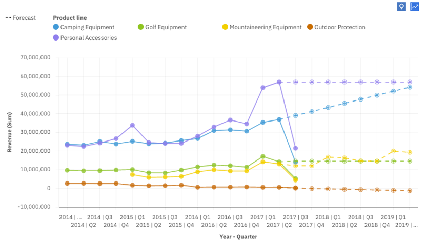
The time series in the charts above correspond to different categories of the Product line. We analyze and discuss each series separately starting with the series Personal Accessories having the highest values, and proceeding with the series displayed below it. 

Each analysis starts with display of an autocorrelation plot. The autocorrelation computes the correlation of a series with lagged versions of itself. If there is high correlation at a specific lag this is evidence of possible seasonal effects. For data that has a trend we difference it in order to remove the trend. Another tool that we use for seasonality detection is the seasonal plot. It displays a line for each seasonal period found in the data.

We compare Cognos Analytics results with Expert modeler feature for automated selection of exponential smoothing models available in the IBM SPSS Statistics. Results from corresponding ETS function in R are not discussed below because a simple exponential smoothing model with no trend and no seasonality is selected for all example series.

Capabilities for three products above are comparable when seasonality period is specified by the user. Each one selects a seasonal exponential smoothing model with specified seasonal period or an appropriate non-seasonal model. Notice that the user is not required to specify seasonal period in Cognos Analytics. Auto setting will select both appropriate seasonal period and a corresponding exponential smoothing model.

Modeling of the considered time series is limited due to small number of observed values. Each series contains only up to 14 time points, one per each quarter over the span of two and a half years.Personal Accessories

CA Forecasting Model

Autocorrelation function of the 1-differenced series on the left and a seasonal plot with period 6 on the right indicate no seasonal pattern. Values are higher towards end of the period during the first 2 cycles, but they become much larger at the beginning of the period in the last cycle.

Cognos Analytics R5 selects a simple exponential smoothing model with no trend and no seasonality. Model fit and residual autocorrelation are acceptable for the simple model displayed below.

Expert modeler in SPSS Statistics selects a more complex model that includes both trend and seasonality with period 4. It fits historic data better than the simple model, but its seasonal pattern does not match the data very well. Seasonal plot for period 4 shows no pattern except for a large increase in Q1 2017. There is no evidence in favor of the more complex seasonal model and the corresponding forecast cannot be trusted.

Camping Equipment

CA Forecasting Model

Autocorrelation function of the 1-differenced series on the left and a seasonal plot with period 5 on the right do not indicate a relevant seasonal pattern. Cognos Analytics R4 uses a very weak and unreliable seasonal pattern. 

Both Cognos Analytics R5 and Expert modeler in SPSS Statistics select the same model with additive trend and no seasonality displayed below.

Golf Equipment

CA Forecasting Model

Autocorrelation function of the 1-differenced series on the left and a seasonal plot with period 4 on the right do not indicate a seasonal pattern. Cognos Analytics R4 picks up a very weak pattern mostly due to increase in the first quarter of 2016 and 2017.

Cognos Analytics R5 selects a simple model with no trend and no seasonality.

Expert modeler in SPSS Statistics selects a more complex model that includes both trend and seasonality with period 4. It corresponds to the model selected in Cognos Analytics R4. Nevertheless, fitted seasonal pattern does not match the data and residual autocorrelation displays a pattern. This model cannot be recommended for forecasting.

Mountaineering Equipment

CA Forecasting Model

Autocorrelation function of the 1-differenced series on the left and a seasonal plot with period 4 on the right indicate a weak seasonal pattern, mostly due to the Revenue increase in the first quarter. Cognos Analytics R4 picks up non-existent signal at 6 lags for series containing 10 observations only. This is due to 4 initial missing values extrapolated from the observed data. Such missing values are simply ignored in Cognos Analytics R5.

Both Cognos Analytics R5 and Expert modeler in SPSS Statistics select the same model type with additive trend and seasonality below. The seasonality with period 4 seems to provide good fit to observed data.

Outdoor Protection

CA Forecasting Model

Autocorrelation function of the 1-differenced series on the left and the seasonal plot with period 4 on the right indicate relatively weak signal at 4 lags, due to increase of Revenue in the first quarter. Cognos Analytics R4 adopts the seasonal contribution, but it is ignored in Cognos Analytics R5.

Trend only model in Cognos Analytics R5 provides a reasonable fit to the data and there are no issues with residuals. However, negative forecast values for Revenue series are not expected, and this model provides no practical value.

Both Cognos Analytics R4 and Expert modeler in SPSS Statistics select the same model type with additive trend and seasonality displayed below. The seasonality seems to provide a plausible fit to observed data. Forecast is also more realistic than for the model above because it remains in the positive range.

Accidents data

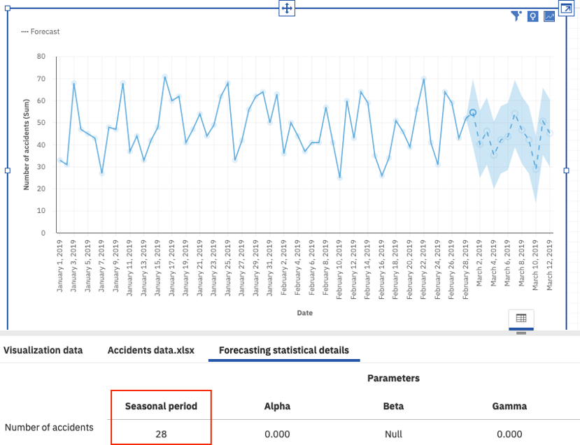
Accidents data contains count of traffic accidents reported daily from January 1, 2019 to February 28, 2019. This data provides a time series with 59 observation affording a more thorough investigation compared to very short Go Sales time series.

Cognos Analytics R4 forecasting algorithm selects a model with large seasonal period 28, while a simple model with no seasonality and no trend is selected in Cognos Analytics R5 instead.

Before (Cognos Analytics R4)

After (Cognos Analytics R5)

Seasonal period: 28 days

Autocorrelation function plot shows that there is a weak seasonal period possible at 28 days. Seasonal plot reveals that two full 28 days periods are somewhat comparable, but they do not present a clear pattern.

Seasonal model with period 28 fits the observed data better than the alternative simple model. However, fitting a seasonal model with additional 28 parameters to the data containing only 59 points greatly increases its chance of overfitting the observed data.  Relatively large number of parameters penalizes the value of Akaike information criterion, and it makes seasonal model a weaker forecasting candidate than the simple model. 

The following table compares 1-step ahead forecast errors for the last 3 observed points using only earlier data for modeling in each instance. There is no advantage in using a seasonal model over a simple model based on (absolute) differences of observed and forecast values.

Forecast Error Comparison

Notice that earlier points cannot be forecasted using a seasonal model with period 28 days because modeling seasonal data minimally requires observing two seasonal periods.

Seasonal period: 7 days

The autocorrelation function plot above shows that possible weekly pattern is detected. Weekly pattern is plausible for Accidents data and we display a seasonal plot and the corresponding box plot for period 7 to further assess its relevance. It turns out that there is a visible pattern where days 5 (Thursday) and 6 (Friday) tend to have higher values, while days 7 (Saturday) and 1 (Sunday) usually have lower number of accidents.

The following charts displays observed Accidents data and fitted values based on a seasonal model with period 7 obtained using forecasting algorithm in Cognos Analytics R5.

Fitted seasonal patterns strongly matches data during the first two weeks, but it becomes considerably weaker towards the end of the series due to the changing weekly pattern of the data.

Again, improved model fit achieved by the seasonal model is not sufficient to overcome the parameter penalty due to estimating 7 additional parameters in the seasonal model. The following table shows it has no advantage in forecasting the last three observed data points.

Forecast Error Comparison

When comparison is extended to earlier points, the seasonal model reduces forecast error by 10% on average compared to the simple model. This indicates overall accuracy advantage for the seasonal model, but the simple model still provides robust forecast for Accident data.

Expert modeler in SPSS Statistics prefers a seasonal exponential smoothing model with period 7 to a simple exponential smoothing model due to a stronger seasonal fit for the observed data. Notice that its seasonal pattern for fitted values does not change over time.

Still, forecast error for seasonal model in SPSS Statistics is not improved when compared to the seasonal model generated in Cognos Analytics. This points to risks of forecasting using a weak seasonal model in practice. Seasonal indices can easily change during future forecast periods.