Build RAG with Visual Grounding with IBM watsonx.ai, Docling and watsonx.data Milvus
Introduction
In the era of ever-expanding digital documents, extracting precise, context-rich answers from large PDF files is a growing challenge—especially when those answers are buried in Tables, Images, Links, Unstructured text. This is where Retrieval-Augmented Generation (RAG) systems come in, combining semantic search and large language models (LLMs) to retrieve relevant information and generate human-like responses.
But what if we could go a step further—not just retrieve and summarize information, but also visually ground it in the original document? That’s exactly what we explore in this tutorial.
What is Docling?
Docling is IBM's open-source toolkit designed to simplify document processing. It adeptly parses diverse formats—including PDFs, DOCX, XLSX, HTML, and images—into structured, machine-readable formats like JSON and Markdown. Docling's advanced PDF understanding capabilities encompass page layout analysis, reading order determination, table structure recognition, and more. With a command-line interface and Python API, Docling integrates seamlessly with generative AI frameworks, facilitating the transformation of complex documents into data suitable for AI model customization and grounding.
-
Supports diverse document types: Handles PDFs, DOCX, TXT, scanned images (OCR), and more.
Visual Grounding RAG System – Execution Overview
The Visual Grounding RAG (Retrieval-Augmented Generation) system implements an intelligent document processing pipeline that not only answers queries but also provides visual evidence by highlighting the exact locations in source documents that support the generated responses.
1. Document Ingestion & Chunking
IBM’s Docling framework processes PDF documents (from URLs or local sources), extracting structured content and breaking it into semantically meaningful chunks. Each chunk preserves layout details, page numbers, and spatial metadata—crucial for visual grounding later.
2. Semantic Embedding Generation
You can choose any embedding model from watsonx.ai. The choice of embedding model is also responsible for determining the accuracy during retrieval. Here text chunk is embedded into a 384-dimensional vector using the SLATE-30M model from IBM watsonx.ai. The embeddings capture the semantic meaning of the content, enabling accurate and meaningful retrieval.

3. Vector Storage & Similarity Search
The generated embeddings are stored in a Milvus vector database, optimized for high-performance retrieval. Here we have used a top-3 similarity search, this is configurable based on use case to get optimal results. This is performed using L2 (Euclidean) distance to find the most relevant document chunks for any given user query.
4. Context-Aware Answer Generation
The retrieved chunks are passed to IBM’s Granite-3-3-8B-Instruct LLM. It generates well-structured answers based on the retrieved context, following a multi-step reasoning style and matching the original document tone.
5. Visual Grounding & Highlighting
Using metadata from the chunks, the system maps the answer back to the exact source pages. Bounding boxes are rendered over the corresponding areas in the original page images, offering visual proof for the generated responses.
Step-by-Step Implementation
Create Milvus Instance on watsonx.data
Set up a Watson Machine Learning service instance and API key
-
Generate an API Key in WML. Save this API key for use in this tutorial.
-
Associate the WML service to the project you created in watsonx.ai.
Setting Up the Environment
In this tutorial, we are using python==3.11.11 Please ensure you're using the same version in case you encounter any discrepancies. First, we'll set up our Python environment and install the necessary packages:
%pip install -q --progress-bar off --no-warn-conflicts langchain-docling langchain-core langchain_milvus langchain matplotlib pymilvus docling ibm-watsonx-ai
1.Data Preparation with Docling
To build an effective Visual Grounding RAG pipeline, we first need to ingest, convert, and structure our source documents.
1.1 Configure the Docling PDF Converter
We initialize the `DocumentConverter` from Docling, specifying options such as:
- Enabling page image generation (useful for visual QA)
- Scaling images for better layout resolution
from docling.datamodel.base_models import InputFormat
from docling.datamodel.pipeline_options import PdfPipelineOptions
from docling.document_converter import DocumentConverter, PdfFormatOption
converter = DocumentConverter(
InputFormat.PDF: PdfFormatOption(
pipeline_options=PdfPipelineOptions(
generate_page_images=True,
)
1.2 Convert PDFs and URLs to Docling JSON Format
from tempfile import mkdtemp
# To use a local PDF, simply provide its path as a string, like: "path/to/local/file.pdf"
doc_store_root = Path(mkdtemp())
dl_doc = converter.convert(source=source).document
file_path = Path(doc_store_root / f"{dl_doc.origin.binary_hash}.json")
dl_doc.save_as_json(file_path)
doc_store[dl_doc.origin.binary_hash] = file_path
json_paths.append(file_path)
1.3 Load Document Chunks via LangChain DoclingLoader
Finally, we use DoclingLoader with ExportType.DOC_CHUNKS to extract hierarchical chunks of text from the structured JSONs. These chunks will be embedded and indexed for semantic retrieval.
from langchain_docling import DoclingLoader
from langchain_docling.loader import ExportType
export_type=ExportType.DOC_CHUNKS
# Note: "Token indices sequence length is longer than the specified maximum sequence length for this model (648 > 512)..." This is a false alarm.
2. Vector generation/Embedding creation
2.1 Authentication Setup
from ibm_watsonx_ai import APIClient
# Set up WatsonX API credentials
"url": "<watsonx URL>", # Replace with your your service instance url (watsonx URL)
"apikey": '<watsonx_api_key>' # Replace with your watsonx_api_key
client = APIClient(my_credentials)
2.2 Generate Dense Embeddings with WatsonX
from ibm_watsonx_ai.foundation_models.embeddings import Embeddings
from ibm_watsonx_ai.metanames import EmbedTextParamsMetaNames as EmbedParams
# Initialize the WatsonX client for embeddings
model_id = client.foundation_models.EmbeddingModels.SLATE_30M_ENGLISH_RTRVR
# Define embedding parameters
EmbedParams.TRUNCATE_INPUT_TOKENS: 128,
EmbedParams.RETURN_OPTIONS: {'input_text': True},
}
# Set up the embedding model
credentials=my_credentials,
project_id="<project_id>", # Replace with your project ID
2.3 Verify Embedding Output
test_embedding = embedding.embed_query(text="This is a test")
embedding_dim = len(test_embedding)
print(test_embedding[:10])
3. Store Embeddings in watsonx.data Milvus
To enable fast and accurate semantic search, we now store our document embeddings in watsonx.data Milvus, IBM's managed vector database. This step initializes a vector store from our Docling-extracted chunks and embeds them using the selected watsonx.ai embedding model.
from tempfile import mkdtemp
from langchain_milvus import Milvus
vectorstore = Milvus.from_documents(
collection_name="docling_demo",
"index_type": "FLAT", # Type of index
"metric_type": "L2" # Required: distance metric
},
"uri": "https://<hostname>:<port>",# Replace with your watsonx.data Milvus URI or IP
"secure": True, # Set True if TLS is enabled
"server_pem_path": "/path_to_ca.cert"
print("connected")
4.Query, Generate Answers & Visualize with Visual Grounding
In this final stage, we perform the core of retrieval-augmented generation (RAG) using:
- IBM watsonx.ai for large language model (LLM) inference,
- watsonx.data Milvus via Langchain to orchestrate the RAG pipeline,
- Docling for visual grounding and bounding-box-based highlighting of answers.
We define a custom prompt template, fetch the most relevant document chunks from Milvus, and pass them to the LLM for answer generation. Finally, we visualize the provenance of the answer using page-level image highlighting.
4.1 Set up watsonx.ai Language Model
from ibm_watsonx_ai.foundation_models import ModelInference
from langchain_ibm import WatsonxLLM
# Initialize model inference
model_inference = ModelInference(
model_id="ibm/granite-3-3-8b-instruct", # Use a watsonx.ai foundational model
credentials=my_credentials,
project_id="<project_id>", # Replace with your project ID
# Wrap with LangChain's WatsonxLLM
llm = WatsonxLLM(watsonx_model=model_inference)
4.2 Define Prompt, Setup Retriever & Execute RAG
In this step, we prepare the core RAG (Retrieval-Augmented Generation) logic:
- Prompt Template: A structured prompt is defined to instruct the LLM to generate a well-explained answer based on the retrieved context.
- Retriever Setup: We configure the Milvus vector store to return the top-3 relevant document chunks for the given query.
- RAG Execution: The retrieved documents are formatted and passed to the IBM watsonx.ai LLM to generate the final answer.
import matplotlib.pyplot as plt
from PIL import ImageDraw
from langchain_core.prompts import PromptTemplate
from langchain_core.output_parsers import StrOutputParser
from langchain_core.runnables import RunnablePassthrough
from docling.chunking import DocMeta
from docling.datamodel.document import DoclingDocument
PROMPT_TEMPLATE = """Generate a summary of the context that answers the question. Explain the answer in multiple steps if possible.
Answer style should match the context. Ideal Answer Length 5-12 sentences.
prompt = PromptTemplate(template=PROMPT_TEMPLATE, input_variables=["context", "question"])
# --- Setup Retriever ---
retriever = vectorstore.as_retriever(search_kwargs={"k": 3})
# --- Helper Function ---
return "\n\n".join(doc.page_content for doc in docs)
def clip_text(text, threshold=100):
return f"{text[:threshold]}..." if len(text) > threshold else text
query = "What is the Percentage of Train data for Section-header?" # Replace with the query of your choice
docs = retriever.get_relevant_documents(query)
formatted_context = format_docs(docs)
response = llm.invoke(prompt.format(context=formatted_context, question=query))
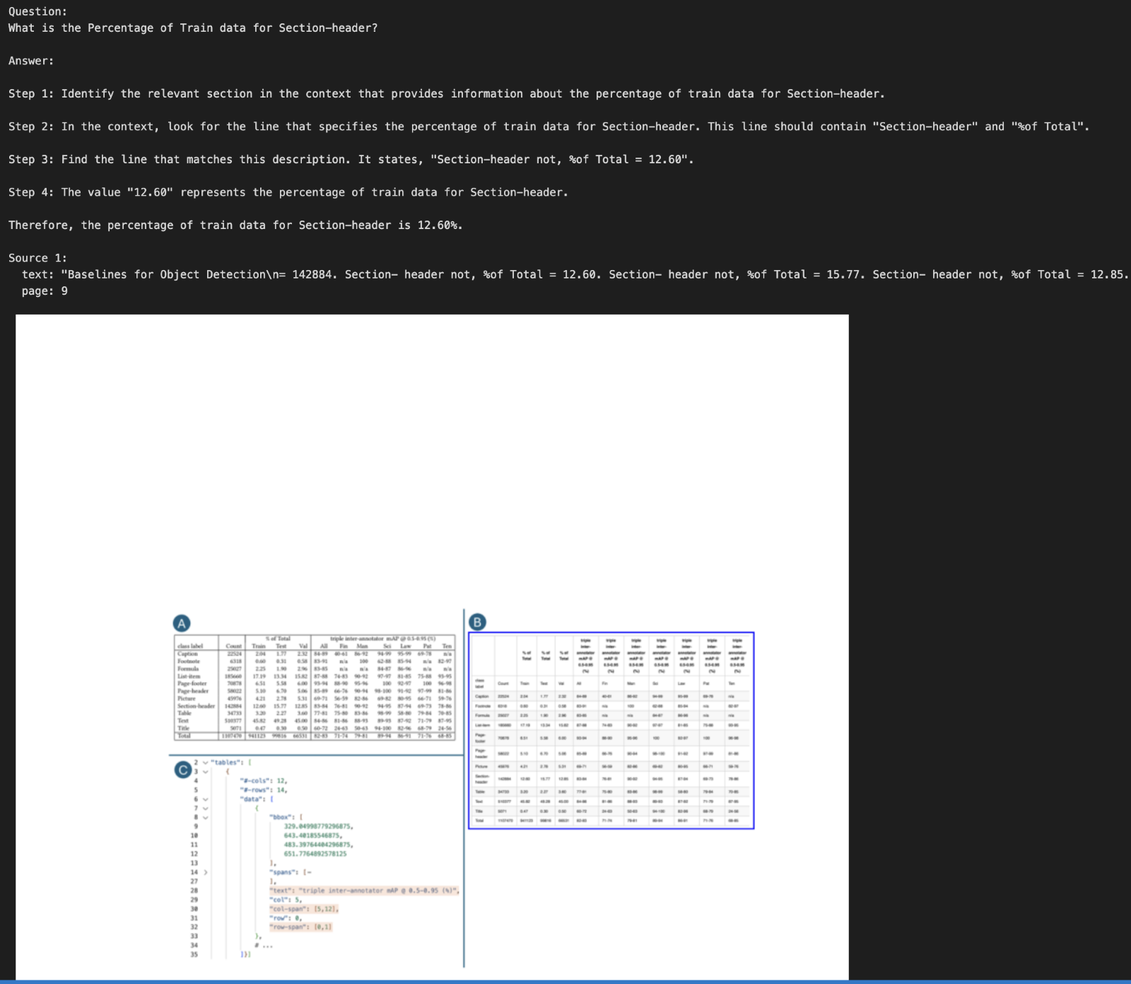
4.3 Visualize Highlighted Context from Retrieved Documents
This section visualizes the parts of the documents that contributed to the generated answer:
1. Build response: Store the query, LLM answer, and retrieved documents in a dictionary.
2. Loop through documents: Print a snippet of each document used as context.
3. Validate metadata: Extract provenance data to locate the exact page and position.
4. Draw highlights: Use bounding boxes to mark the relevant text areas on the page images.
5. Display images: Show the annotated pages using `matplotlib` for visual reference.
# Build response dictionary
print(f"Question:\n{resp_dict['input']}\n\nAnswer:\n{resp_dict['answer']}")
# --- Visualization Code (Docling Highlight) ---
for i, doc in enumerate(resp_dict["context"][:]):
print(f"\nSource {i + 1}:")
print(f" text: {json.dumps(clip_text(doc.page_content, threshold=350))}")
# Validate and load metadata
meta = DocMeta.model_validate(doc.metadata["dl_meta"])
# Load full DoclingDocument from the document store
dl_doc = DoclingDocument.load_from_json(doc_store.get(meta.origin.binary_hash))
for doc_item in meta.doc_items:
prov = doc_item.prov[0] # Only using the first provenance item
if img := image_by_page.get(page_no):
page = dl_doc.pages[prov.page_no]
print(f" page: {prov.page_no}")
img = page.image.pil_image
image_by_page[page_no] = img
bbox = prov.bbox.to_top_left_origin(page_height=page.size.height)
bbox = bbox.normalized(page.size)
bbox.l = round(bbox.l * img.width - padding)
bbox.r = round(bbox.r * img.width + padding)
bbox.t = round(bbox.t * img.height - padding)
bbox.b = round(bbox.b * img.height + padding)
draw = ImageDraw.Draw(img)
# Display all images with highlights
plt.figure(figsize=[15, 15])
Retrieved Response:-

Conclusion
In this notebook, we built a robust and explainable Visual Grounding RAG Pipeline by integrating semantic retrieval, large language models, and visual document understanding.
-
Semantic Retrieval
Milvus was used to fetch the most relevant document chunks, enabling accurate and context-aware responses.
-
Answer Generation
IBM watsonx.ai’s Granite-3B model generated insightful answers grounded in the retrieved context.
-
Visual Grounding
With IBM’s Docling, we extracted metadata and bounding boxes to visually highlight answer locations, adding transparency.