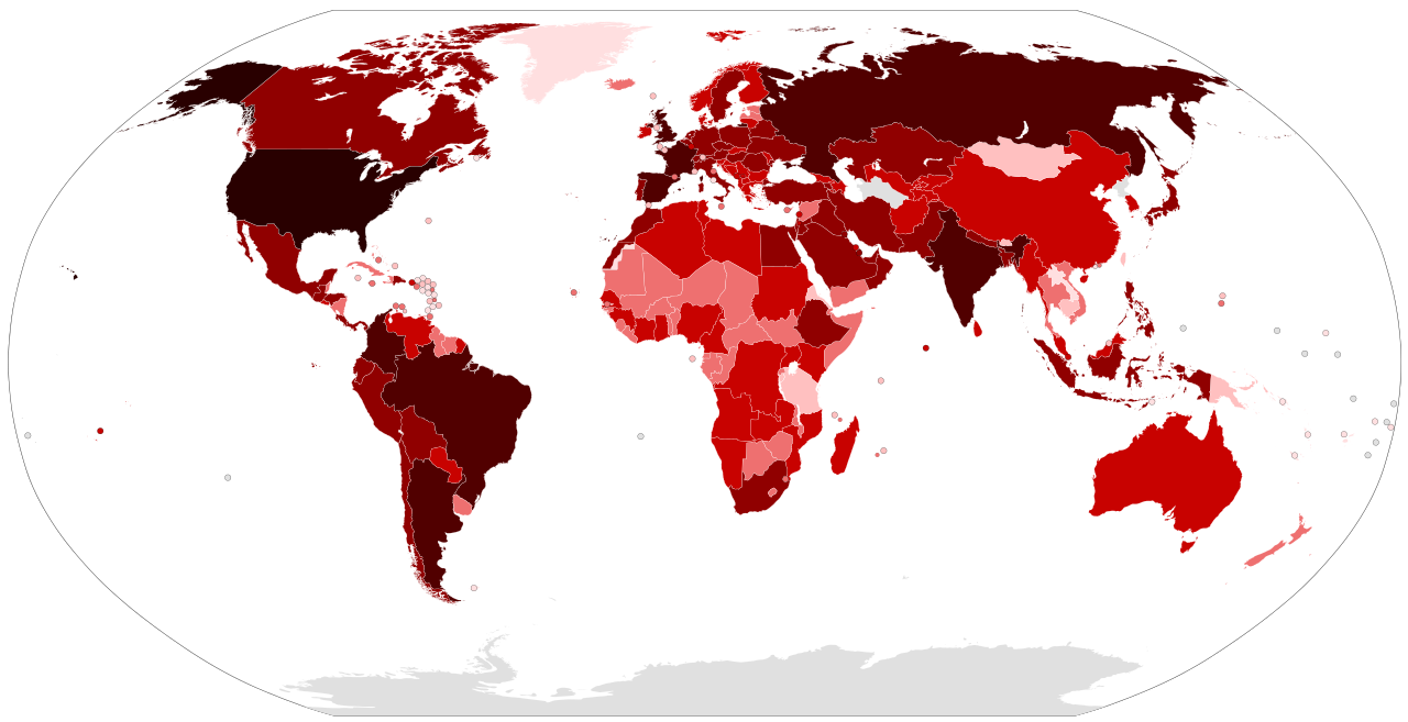
 Photo by Pharexia on Wikipedia
At present, we are experiencing a pandemic that is leaving approximately 1.3 million deaths worldwide, the changes produced by Covid-19 or commonly called coronavirus have impacted several countries in terms of politics, health, education, among others. That is why, since it is a current issue, it is necessary to constantly update this information. On the other hand, thousands of comments are created per second in the different social networks such as Facebook, Linkedin, Instagram, and Twitter and they communicate opinions, feelings, and concerns of the thousands of users of the respective social networks. The immense amount of data well used would allow us to understand the behavior of people, the facts and thus be able to take action.
 Imagen extraída de Twitter
Currently, there are specialized architectures that can parse the comment in its original form (of course after the comment is cleared). These architectures are recurrent neural networks (RNN) and are of various types such as one to many (generally used for image captioning), many to one (used for the classification of feelings), and many to many (used for translators generally ).
A type of RNN, called Long-Short Term Memory (LSTM) has memory units that allow you to learn the dependence of the order between elements in a sequence and the context necessary to make the classification or prediction (time series forecasting).
LSTM
 Photo by isch_tudou on Jianshu
BiLSTM
Methodology
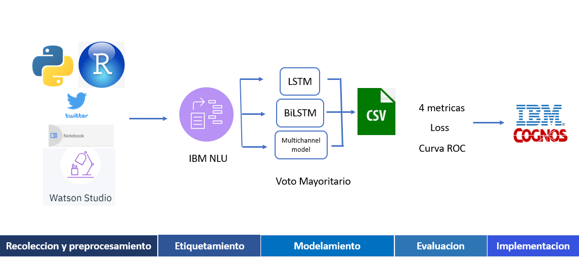
The methodology consists of 5 steps: data collection and preparation, labeling, modeling, model evaluation, and model implementation.
Data collection and pre-processing
For the collection, the tweepy and twitterR library was used in order to get comments with the keywords: coronavirus, covid19, cuarentena y los hashtags #coronavirus, #covid-19, #bonouniversal, #yomequedoencasa, #cuarentenaextendida, #toquedequeda, #vacuna.
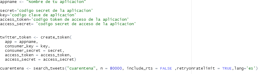
The name of the app and the 4 Twitter developer keys are defined, then an object of the token type is created to perform the extraction of tweets. Subsequently, the tweets are extracted with the search_tweets function that has as parameters:
- keyword → is the word by which the comments will be extracted
- n → indicates the number of comments to extract
- include_rts → indicates if retweets are extracted using a boolean
- retryonratelimit → indicates if the function continues to extract tweets after exceeding the limit (15 min after each extraction)
- lang → indicates the language of the comment
Because twitterR allows to get a higher volume of tweets, it was used in order to get the data for training. These tweets were saved in a csv file.

On the other hand, tweepy was used to automate the extraction of tweets in a Watson Studio Notebook.
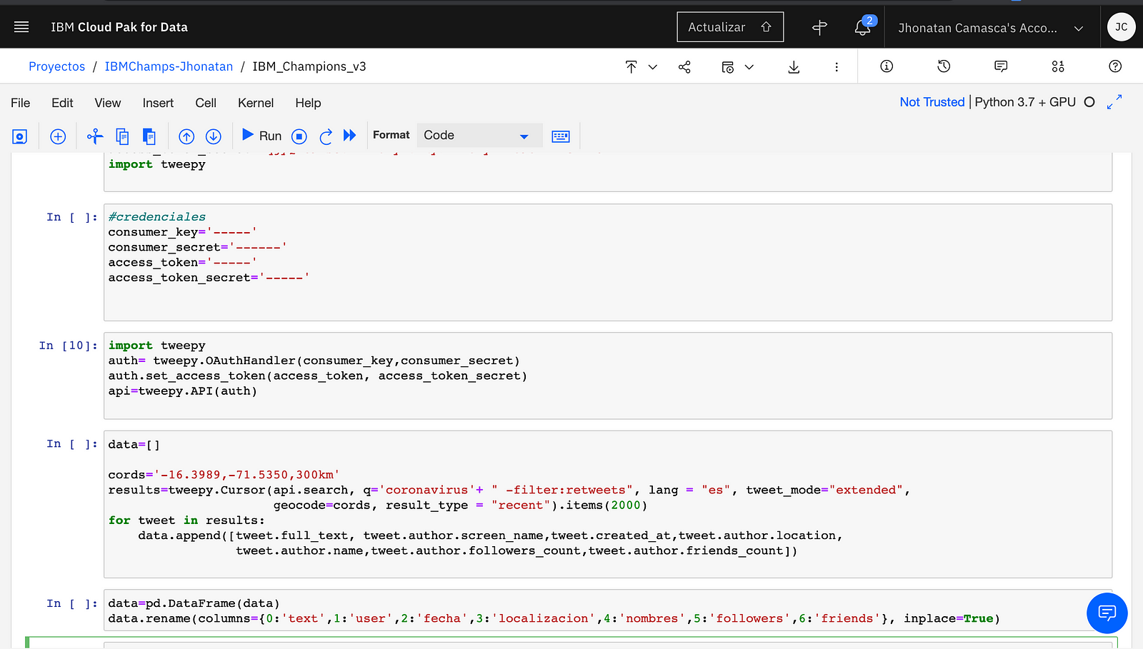
Tweepy is imported in the first cell, then the same credentials used with Rstudio to extract the tweets. To extract the tweets with tweepy you must first use the OAuthHandler function that will receive the consumer codes, then access is given with the set_access_token function and finally with the API function the permission for the extraction of tweets is enabled.
The Cursor function is the one that will allow us to extract the tweets and has as parameters:
- q → is the keyword or ‘query’ to extract the tweets.
- lang → the language of the tweets.
- tweet_mode → by default is None, if ‘extended’ is used it will allow to bring more than 140 characters.
- geocode → allows extracting tweets from a certain place based on their coordinates and a diameter of 250km.
- result_type → ‘recent’ indicates that recent comments will be extracted
- items → is the number of comments.
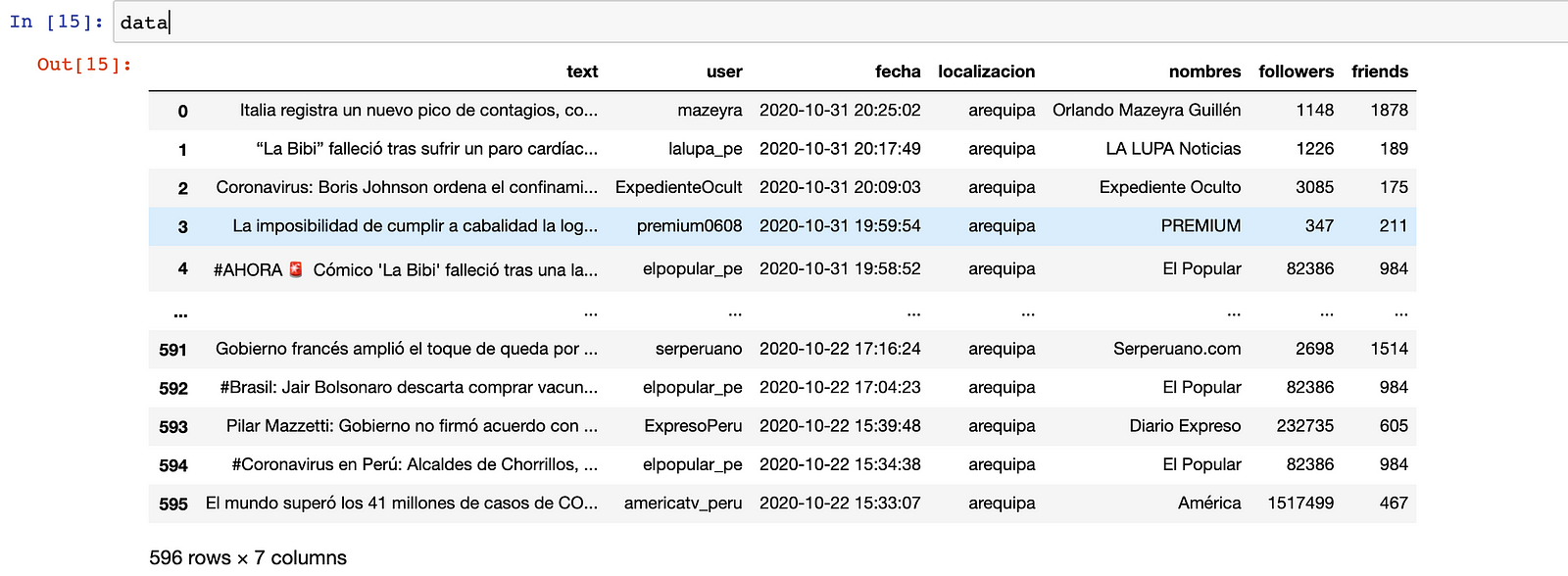
All the information is saved in results and using a for loop the information obtained in each element is disaggregated. The data extracted was the tweet, the user, the date, location, user name, number of followers and number of friends.
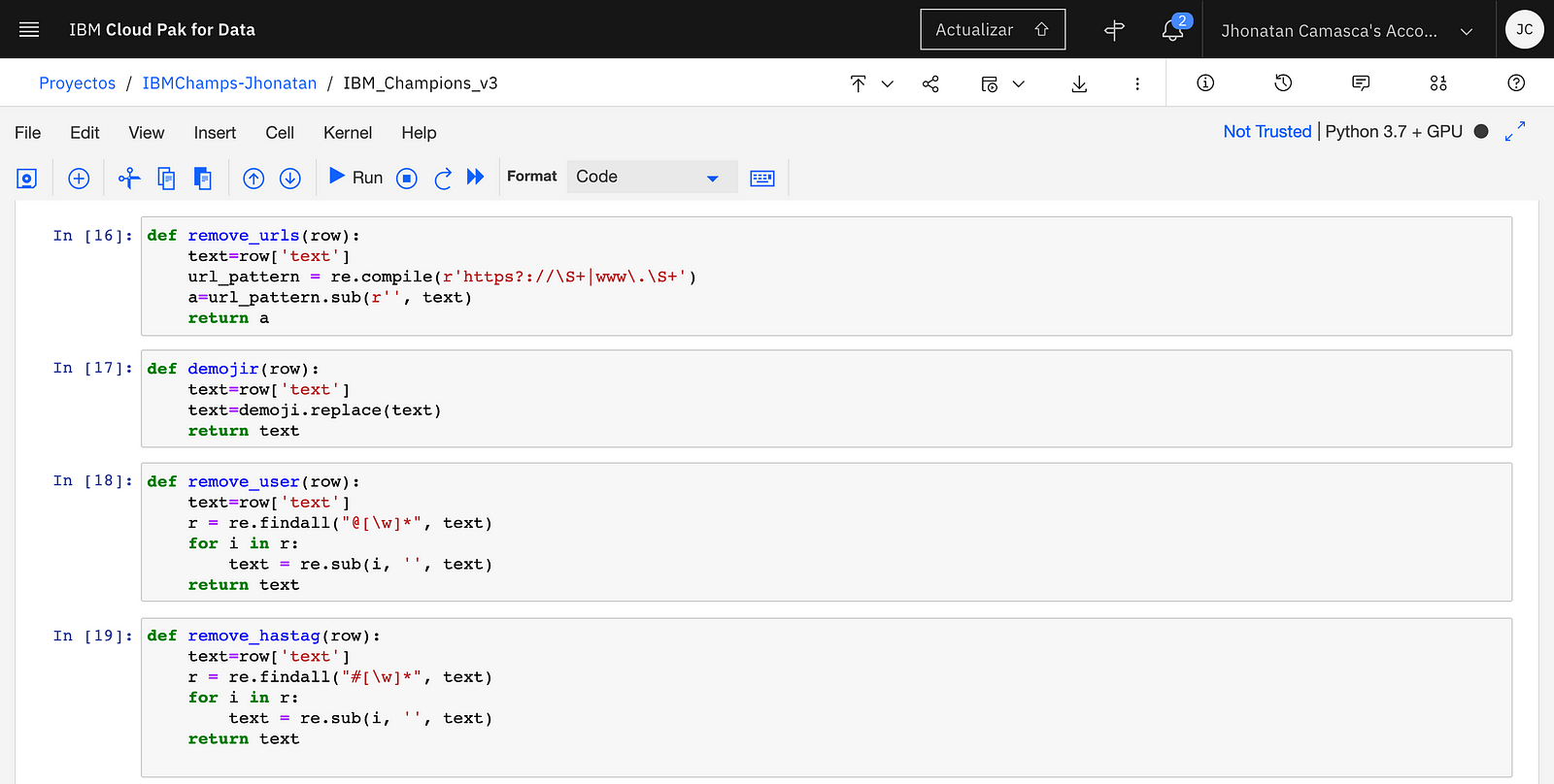
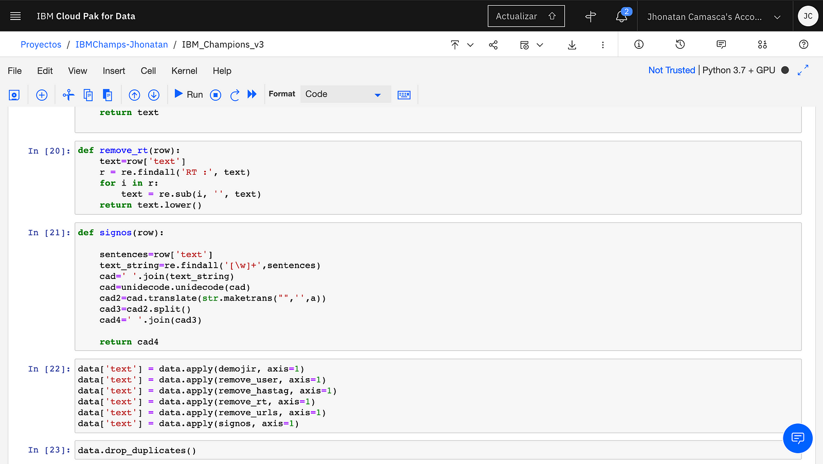
Subsequently, the comments are preprocessed, using the functions remove_urls, demojir, remove_user, remove_hashtag, remove_rt and signs in order to remove the urls, emojis, hastags, RTs (from the retweets), and the signs and tildes are removed.
With the apply function, the functions are applied to the dataframe. Finally, the duplicates of the dataframe were removed with the drop_duplicates () function.
Labeling
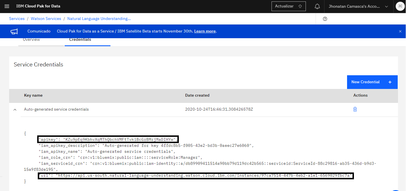
To label the data, the IBM Cloud service, Natural Language Understanding (NLU) was used. The information necessary to use this service is the apikey and the url.
Once an NLU service is created, a Notebook is opened for labeling. To do this, the NaturalLanguageUnderstandingV1, IMAuthenticator, SentimentOptions and KeywordsOptions functions are imported.
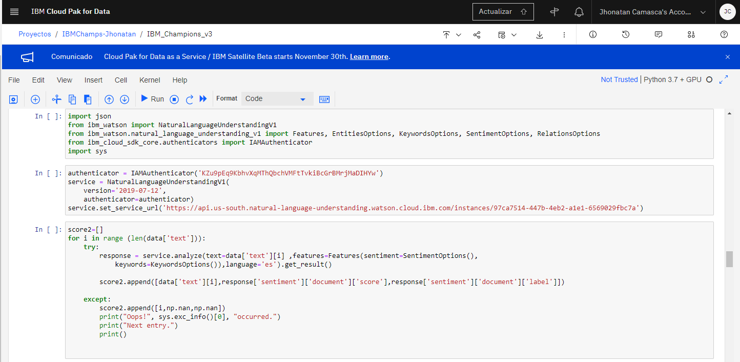
To use the service within the Notebook, an authenticator is created with the apikey. A service is created using the authenticator and the version. Then this service is activated giving the url as input. Subsequently, through a for loop, each comment is analyzed and its polarity is obtained (the api gives you three polarities: positive, negative and neutral), the score (percentage of confidence that it is that polarity) and the same comment, saving them in a list.
Then the comments are filtered with more than 90% confidence, these being tagged by hand in order to create a more precise classifier.
Modeling
It should be noted that before being able to train deep learning architectures, keras == 2.4.3 and tensorflow == 2.3.0 of the following must be installed, using the following commands:

In this post only deep learning architectures called:
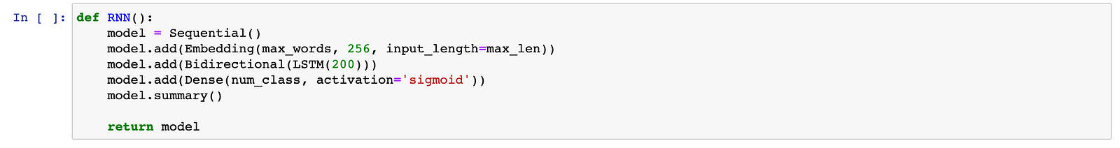
- BiLSTM: Bidirectional Long- Short Term Memory is a recurrent neural network that, unlike LSTM, allows us to learn from both past and future information and better contextualize the information.
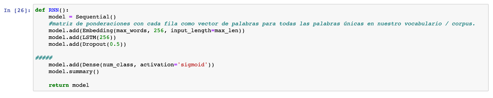
- LSTM: Recurring neural networks that are explicitly designed to avoid the long-term dependency problem and are able to remember information for long periods of time is practically their default behavior.
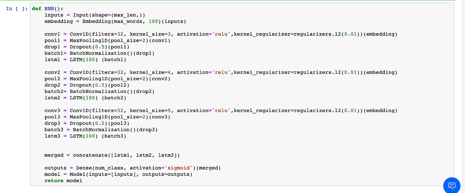
- Multichannel (multichannel): it is an architecture that uses multiple convolutional 1-D (one-dimensional) networks in parallel that have different kernel sizes
Paso 1: Importing libraries
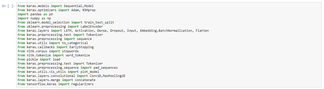
The libraries that will be used were NumPy and pandas for the manipulation of the textual data. On the other hand, the models, optimizers, layers, preprocessing, convolutional, regulizers, and merge libraries were used to create the 3 different deep learning architectures and optimize them with the optimizers: Adam, RSMprop, SGD.
Paso 2: X and Y split
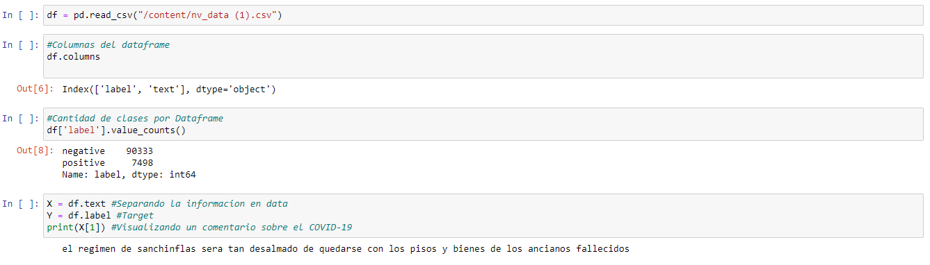
Then the tweets are read using pandas. As you can see we have unbalanced data and it is because in reality, the number of negative comments is greater than the positive ones, this being the real distribution of the tweets.
Paso 3: One-hot encoding

With the LabelEncoder function, the one-hot encoding will be performed to be able to convert the positive and negative labels into 0 and 1.
Paso 4: Train-Test split
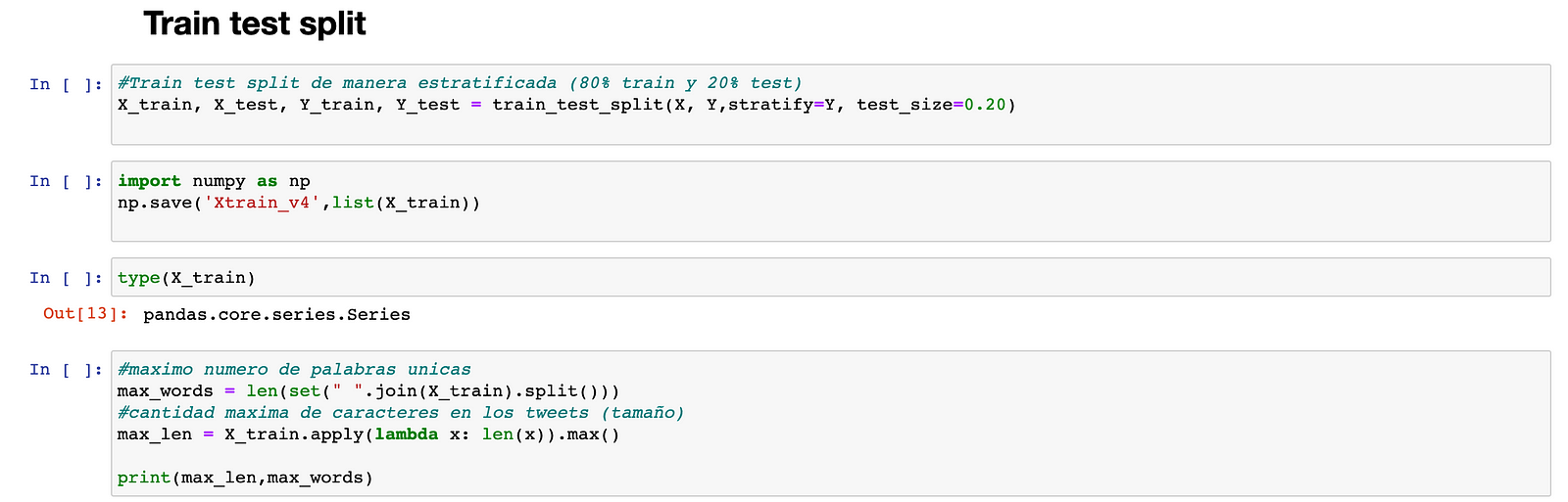
Then, the 80/20 split train-test is performed, the number of unique words, and a maximum number of characters in all tweets are calculated. It should be noted that the stratify parameter was used to perform a division that has the proportion of values in the sample produced at the time of the split.
For example, if the variable y is a binary categorical variable with values 0 and 1 and there are 25% zeros and 75% ones, stratify = y will ensure that your random division has 25% zeros and 75 % of ones in the training data (X_train) and test (X_test).
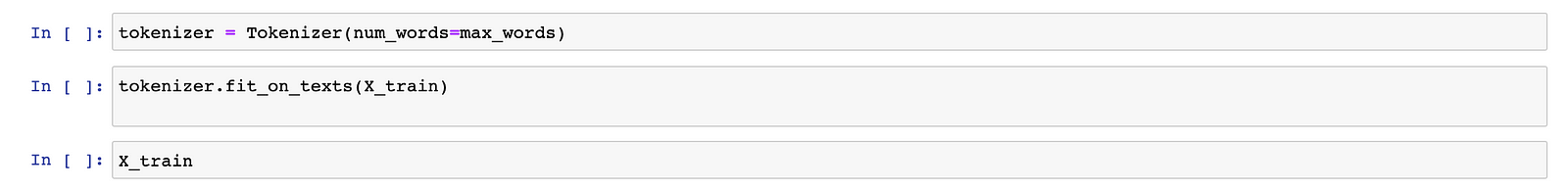
Using Tokenizer, a text corpus was vectorized with the maximum number of unique words, that is, our dictionary has the maximum size of unique words, converting each text into a sequence of integers (each integer is the index of a token in a dictionary).

It should be noted that for Tokenizer to convert tweets to a list of entire sequences that encode the words, the function texts_to_sequences must be used.

This function transforms the list of sequences obtained after using the texts_to_sequences into a Numpy 2D array of the form (max_words, max_len) maxlen is the length of the longest sequence in the list.
Paso 5: Deep learning architectures
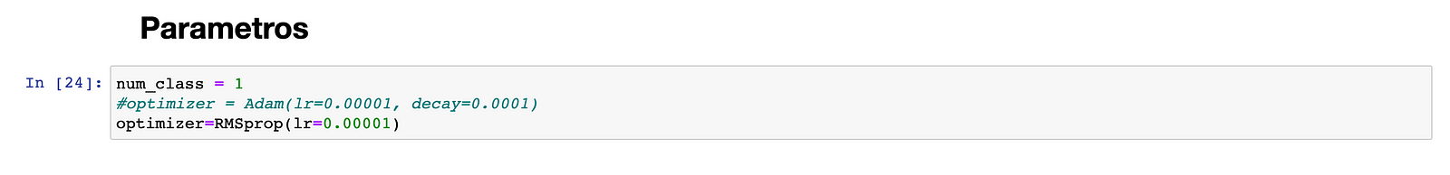
The parameters are num_class = 1, since it is a binary classification and from all the optimizers a better performance was obtained with the RSMprop with a learning rate of 0.00001
The architectures are 3:
LSTM
BiLSTM
Multichannel model
Later the respective architectures are loaded.

Paso 6: Compiling the architectures

Of the three optimizers (SGD, Adam and RSMprop) the one that gave us the best results was the RSMprop
Paso 7: Training the architectures

Different amounts of epochs were used due to the nature of the architectures.
From the Multichannel architecture, it can be seen that the model generalizes fast and tends to overfit fast.
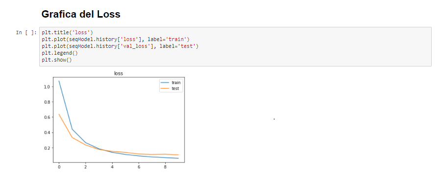
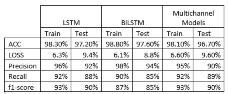
We can see that in general we have a good performance from the three models and that they have generalized the dataset information relatively well.
To proceed with the Majority Voting technique, both the Tokenizer and the h5 models must be exported

Majority Voting
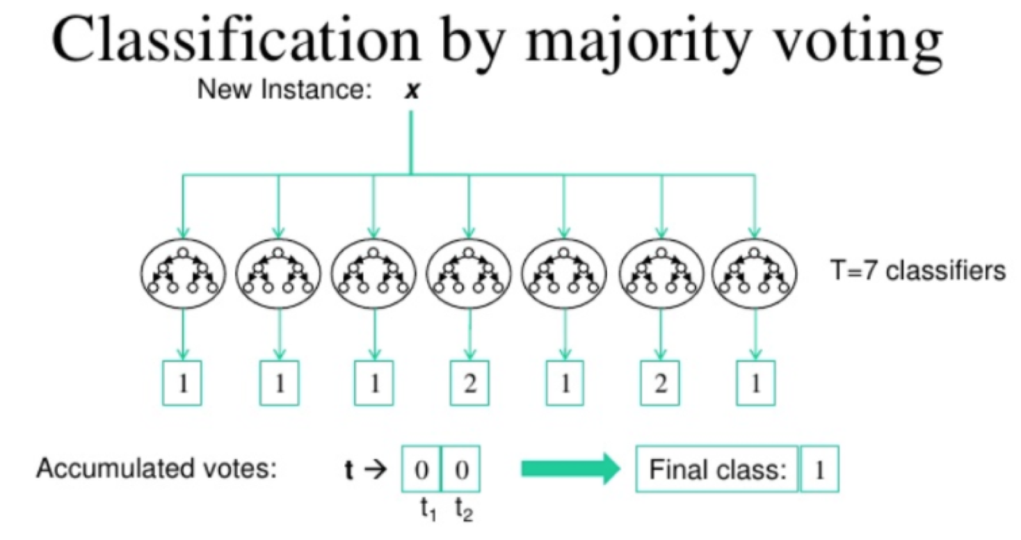
Photo by Suarez(2012) on O’Really
The Majority Vote technique implies that the classification is by the class with the most votes. That is, if we have 5 classifiers, let’s take the mode obtained from all the 5 results.

First, we must import the project credentials.
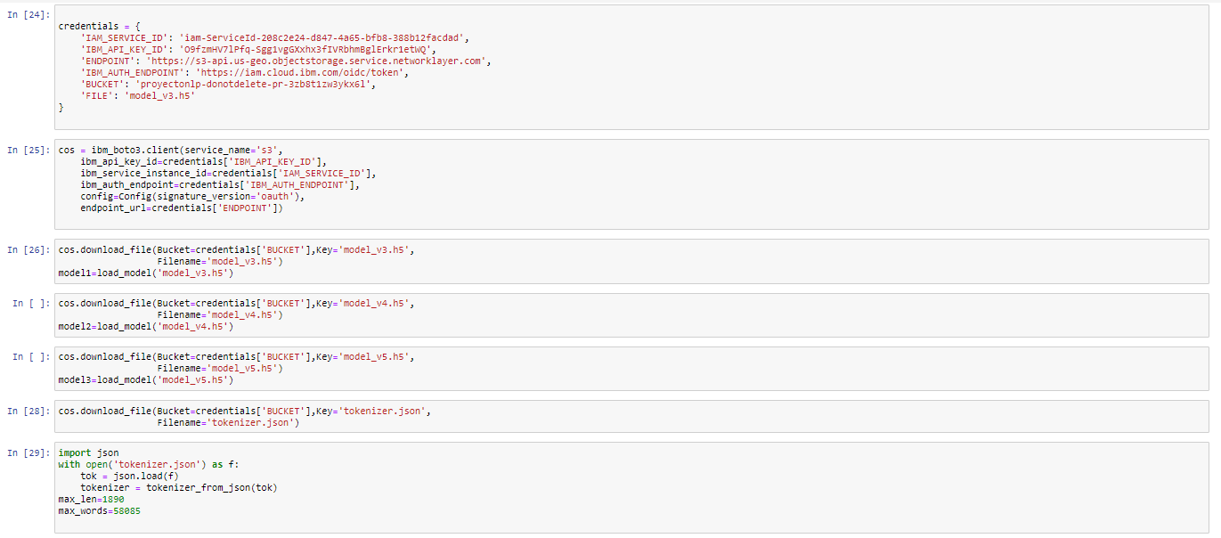
Then the model credentials are imported and through the ibm_boto3 and download_file functions we can make use of the three deep learning architectures (model_v3, model_v4, model_v5). It is very important that we also import the tokenizer since it contains the list of words from the dictionary with their respective index and it will be necessary to make the prediction.
Mayority Voting Code
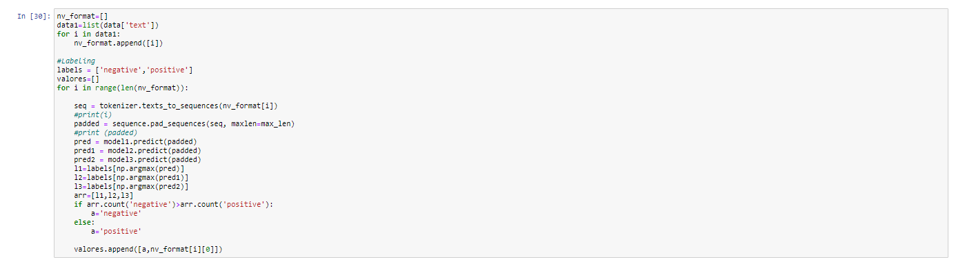
In the code, the predictions are saved in pred1, pred2, pred3 and the labels are obtained through argmax. Afterwards, the classes are stored in an array in order to determine which classes have the most votes and by means of an if, get the majority vote. Those comments will be saved in a csv to be saved in the Object Storage and with IBM Cognos deploying the dashboard.
Implementation
Within the IBM Cloud Pak for Data there is an asset called IBM Cognos Dashboard Embedded, which is an API-based solution that allows developers to easily add end-to-end data visualization capabilities to their applications. Therefore, it was used to graphically display the results, prediction and insights that were found in the data extracted from Twitter.
The dashboard was divided into three sections:
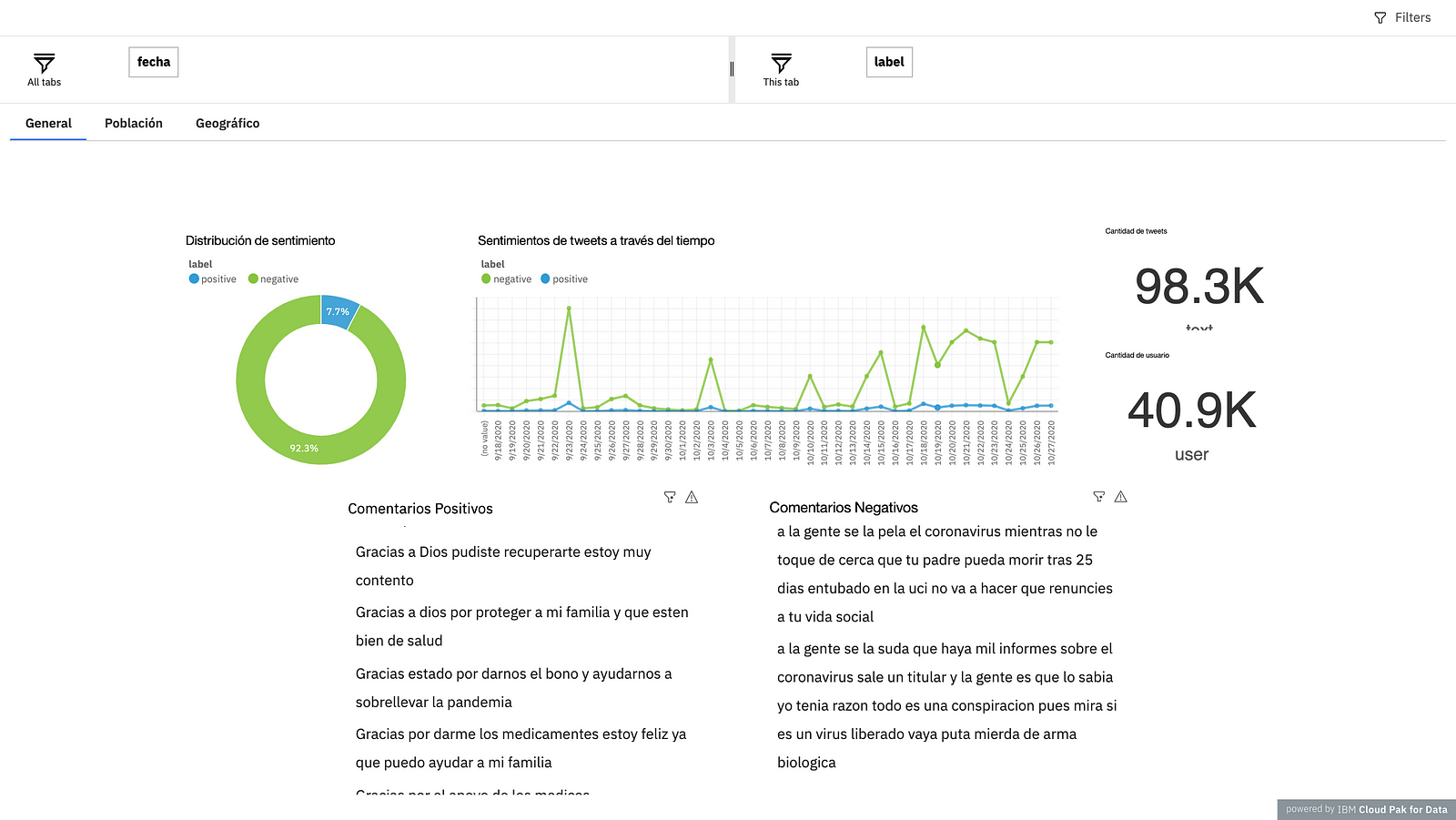
The first, is called “General”, the objective is to show general KPIs, you can see the “Sentiment distribution” graph to see if most of the comments have a positive or negative sentiment. Next, you can see the graph that shows the sentiments of tweets over time, the purpose of which is to be able to identify whether for each new post the comments are having positive or negative effects. Then, there are two numbers that indicate the amount of tweets extracted and the number of users, they are two important numbers that allow to know in a “General” way the business model. Finally, at the bottom there are two lists that contain the positive and negative comments.
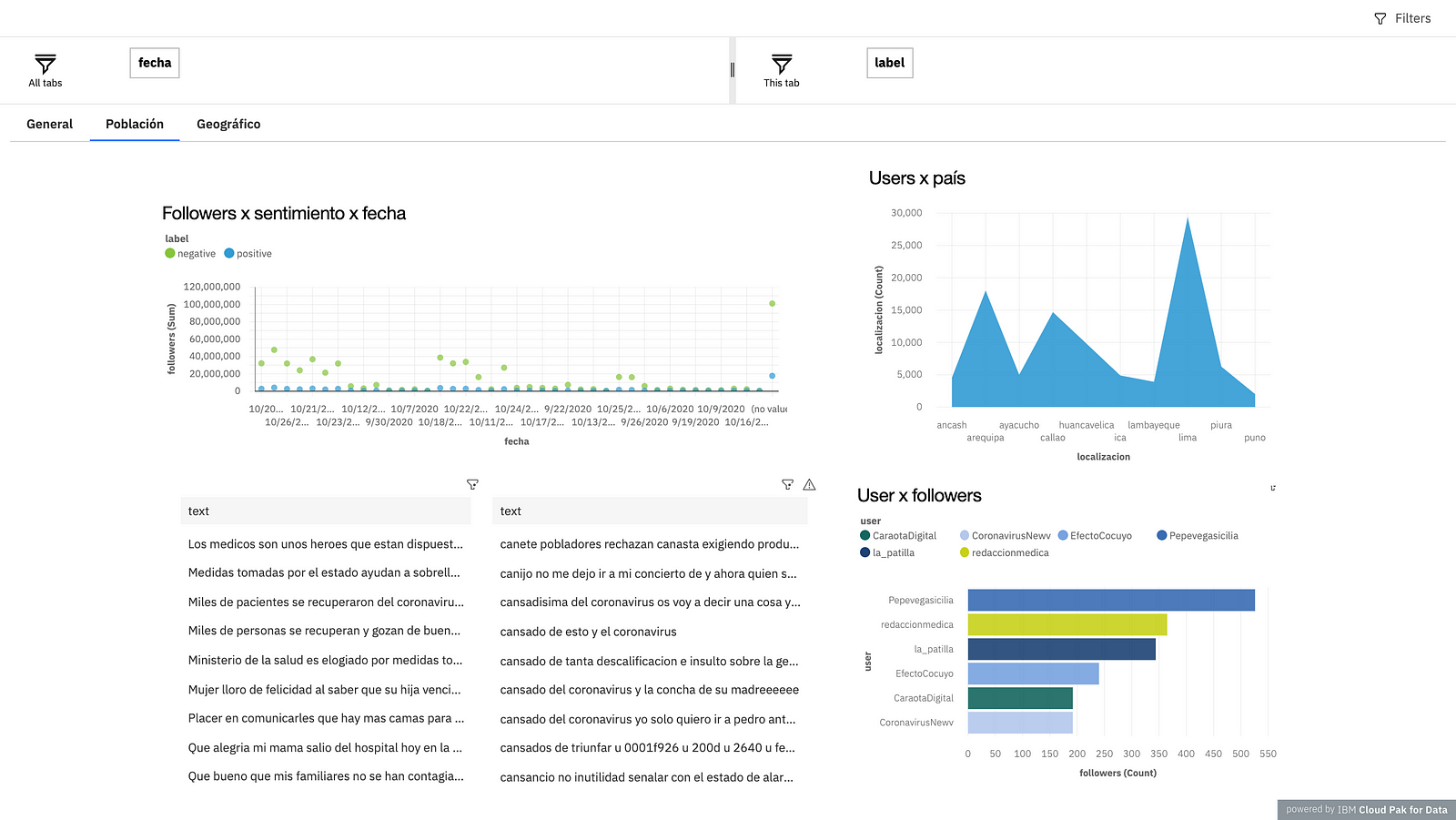
The second is called “Population”, what you want to represent is how are the comments for each user, to be able to make decisions based on the number of followers that a person may have. In the first graph you can see a dispersion visualization, whose objective is to find people who maintain a position against or in favor of the issue and to be able to identify how much influence they have on the networks per day. Next, you see a graph that is divided by the number of users and knowing where they are from, in this case the majority were from Lima. At the bottom, there are the positive and negative comments, unlike the first section, in this section, you can filter the comments at the user level, in order to understand what each one says. Finally, a bar graph is observed, which indicates who are the users who have the highest number of followers and according to this, new strategic decisions can be made.
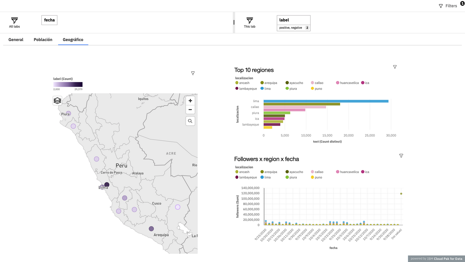
The third, is called “Geographic”, in this case the analysis is through the city in Peru, on the geographic map you can see where this topic is most talked about, the circles represent the place and the intensity of color represents the number of tweets. In the graph “Top 10 regions”, the comparison of the number of tweets per city is observed in greater detail, the cities of Lima, Callao and Piura are those with the highest number of tweets. Finally, in the graph “Followers x region x date”, you can see by date and city, which is the user that has the highest number of followers and know if the tweets he has written are positive or negative.
#GlobalAIandDataScience#GlobalDataScience