Forecasting and prediction are important tasks in real world applications that involve decision making. In such applications, it is important to go beyond discovering statistical correlations and unravel the key variables that influence the behaviors of other variables using an algebraic approach.
If the past values of a set of time series are useful in predicting the future values of one or more time series of interest, then we say they have (Granger) causal relationship. The IBM SPSS Temporal Causal Modeling(TCM) algorithm is designed to discover the key causal relationships in the time series data. Once the users select the time series of interest as targets and the corresponding predictor time series, TCM will build one powerful model system, which includes the causal relationships for every target and its predictors, the model structure as well as model coefficients, which can be used to do the further prediction and visualization.
TCM supports many kinds of use scenarios. Business decision makers can use TCM to uncover causal relationships within a large set of time-based metrics that describe the business. The analysis might reveal a few controllable inputs, which have the largest impact on key performance indicators. Managers of large IT systems can use TCM to detect the anomalies in a large set of interrelated operational metrics. The causal model then provides an approach to discover the most likely root causes of the anomalies. TCM supports two types of data structures, one is column-based data and the other is multidimensional data.
Column-based dataFor column-based data, each time series field contains the data for a single time series. For example, the field Lever1 is one single time series, while the Lever2 is another one. This structure is the traditional structure of time series data.
Multidimensional data
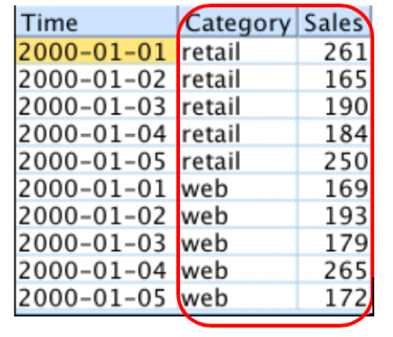
For multidimensional data, each time series field contains the data for multiple time series. Separate time series are identified by a set of dimension fields. For example, the "Sales" field contains data from two different sales channels (retail and web). "Category" is a dimension field with values 'retail' and 'web'.
Note: Currently, only IBM Watson Studio supports multidimensional data. It is not supported by IBM SPSS Modeler or Statistics.
Use Case: Business KPI Monitoring
Enterprises in the information age measure and maintain a large number of metrics in their daily operations. On one hand, this provides the decision maker with rich information sources from which one can potentially obtain useful insights for their business decisions. On the other hand, however, this poses a new challenge, namely, of knowing which metrics to focus on, how to interpret what these metrics mean to the business, and of making decisions on what actions may be needed in response.
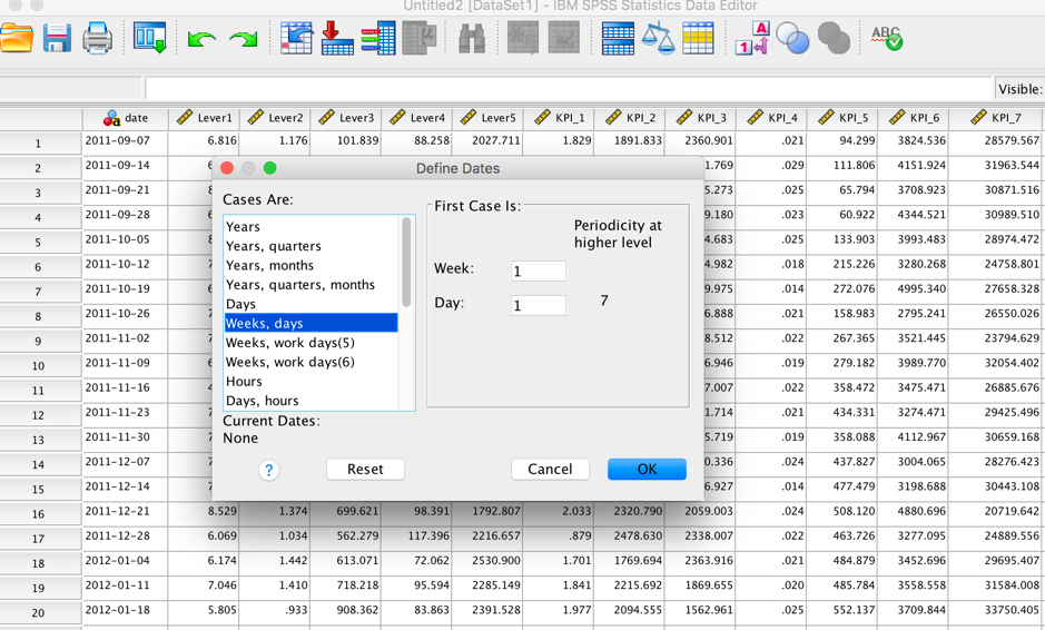
Alex is a decision maker in a company. He gets the data kpi.csv representing the KPIs of the company, where there are 25 KPIs and 5 Levers. KPI_2, KPI_25 and KPI_4 are the profit, cost and the sales of his company, respectively. Other KPIs are related with the domain knowledge and have the special meaning, which are trade secrets. He always asks himself "what metrics are most critical to track and maintain in order to ensure the overall health and success of the company?" and "what metrics should I act upon in order to bring about the maximum overall benefit?". There are many products that can handle these tasks on the market. However, they are too heavy and difficult to use. He heard IBM SPSS has a customized algorithm named TCM for the decision makers which has lots of powerful features to help users do the KPI analysis. He opens IBM SPSS Statistics, and the simple UI and abundant features are very appealing. Before using TCM, Alex defines a date and time variable with Week as the interval for the analysis.
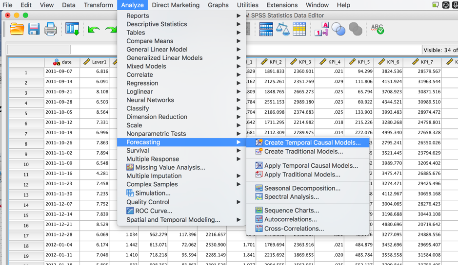
After that, he selects the "Create Temporal Causal Models" in "Forecasting" from the "Analyze" Tab.
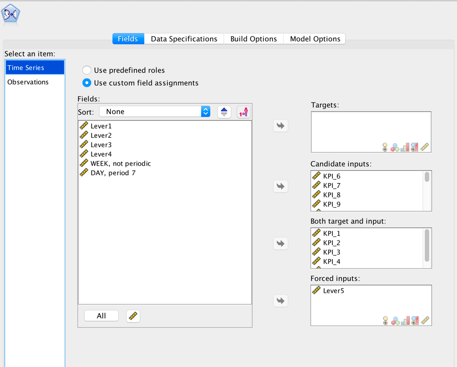
In the Fields tab, Alex selects the option "Use custom field assignments" and chooses KPI_1, KPI_2, KPI_3, KPI_4 and KPI_5 are set to be "Both target and input." Meanwhile, he sets the Lever5 to be "Forced inputs," according to his domain knowledge, which means that they are always included in the selected predictor set. The other KPIs are chosen to be "Candidate inputs," where from which predictors (e.g. Lever1) in the left panel will be selected.
In the Build Options tab, there are some basic settings for TCM modeling and output; each setting has its default value. Alex resets "Maximum number of inputs for each target" to be 8 and "Number of Lags for Each Input" to be 5.

Now, he finishes all the settings and clicks the Run button at the bottom right corner. After the TCM Model is built there is another output page shown.
Bravo, well done! Alex is so excited about how easy it is to use and how rich the output is. He sees the three main parts in the output, Model information, Evaluation and Interpretation.
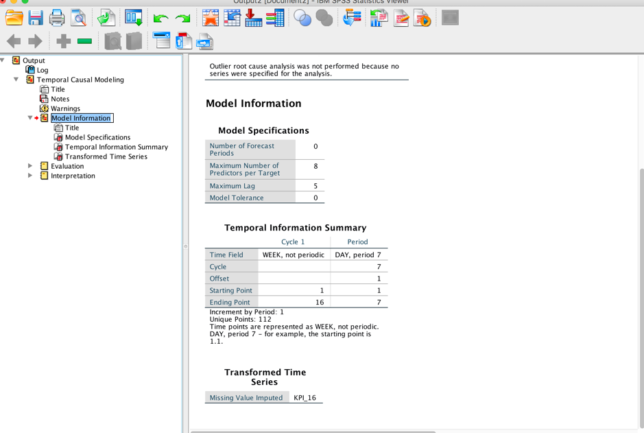
Model Information:
In "Model Specifications", Alex can confirm the settings used in the whole process. He noticed that the time series "KPI_16" is transformed because of the Missing value handling. He likes what he sees and thinks it's great!
Evaluation:
The "Overall Model Quality" shows the distribution of model quality for all the built models. There are many kinds of criteria that can be used to do the evaluation. Alex selects R Square, which is the default criterion; the larger the R Square, the better the model. From the figure, Alex accepts the built models because 80% of the models have R Square values in [0.75, 0.88].
 Alex is also a statistical expert with rich domain knowledge. He wants to know the detailed model effects for further understanding. The Table "Test of Model Effects" shows the F-test and significant values for every target and its predictors. From the table, the KPI_25 (cost), Lever5, KPI_4(sales) and KPI_5 are the most important predictors for the target KPI_2(profit) because all the significant values are lower than 0.05.
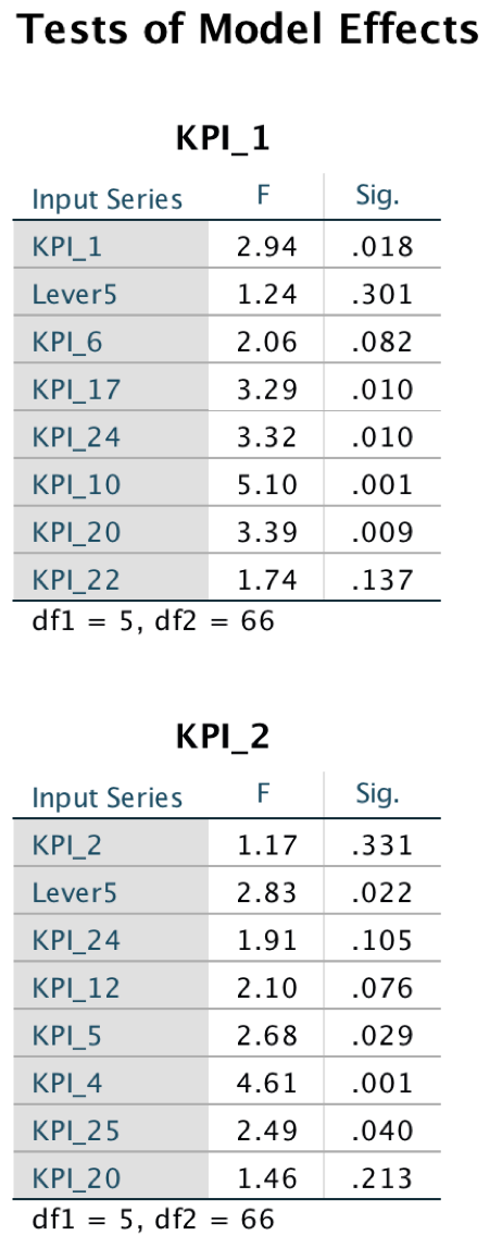
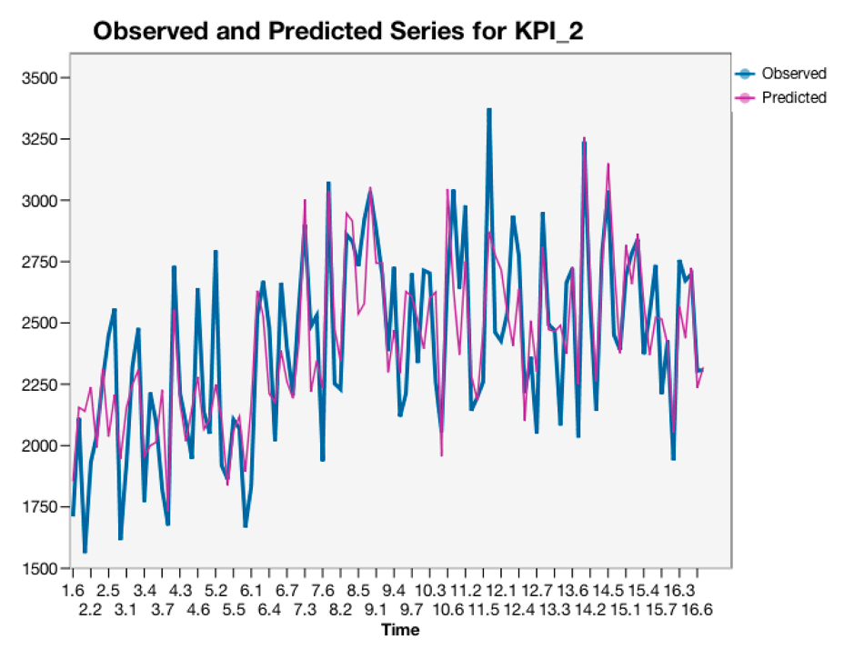
Alex also wants to see the observed and predicted chart for the KPI_2(profit) and check the overall fit performance. Exactly as expected, he sees the "Observed and Predicted Series for KPI_2" in the output. From the chart, the fit is well-behaved. It's another excellent result from his analysis!
Interpretation:
Up until now, only the model information has been shown. Alex wants to see if there is an impact graph to show the relationship between all of the targets and predictors. Yes! There is a graphical representation of the causal relationships among series in IBM SPSS Statistics. The "Overall Model System" shows the relationships among the series with arrows. The Causal relation between two series is measured by an associated significance level, for which a smaller value indicates a stronger connection.
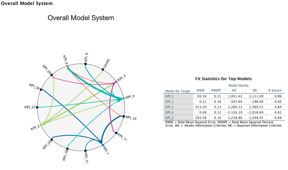 From the chart, Alex gets the same conclusion as he did from the table "Test of Model Effects" in that there are 4 top predictors for KPI_2(profit), which are Lever5, KPI_4(sales), KPI_25(cost) and KPI_5. Besides the "Overall Model System," IBM SPSS Statistics also provides an Impact Diagram, which is a graph representing the Granger causal relationships among the metrics. Using the Impact Diagram, Alex finds that there are lots of Granger causes for KPI_2(profit). Besides the 7 selected predictors in model, there are other impacts such as KPI_19, KPI_3, KPI_21, etc. With this conclusion, Alex can focus on all of the main KPIs that will impact his decision making.
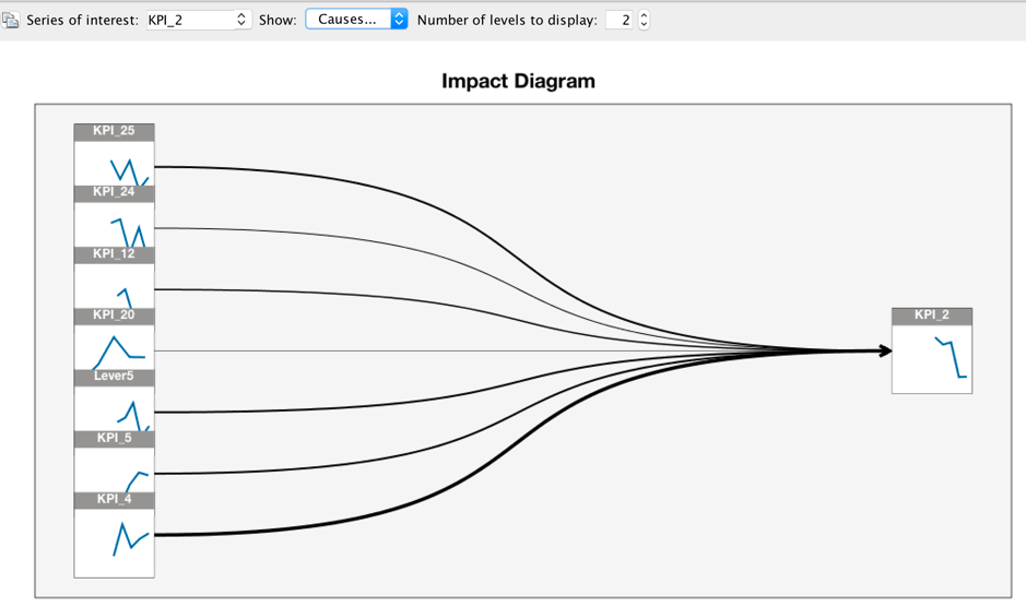
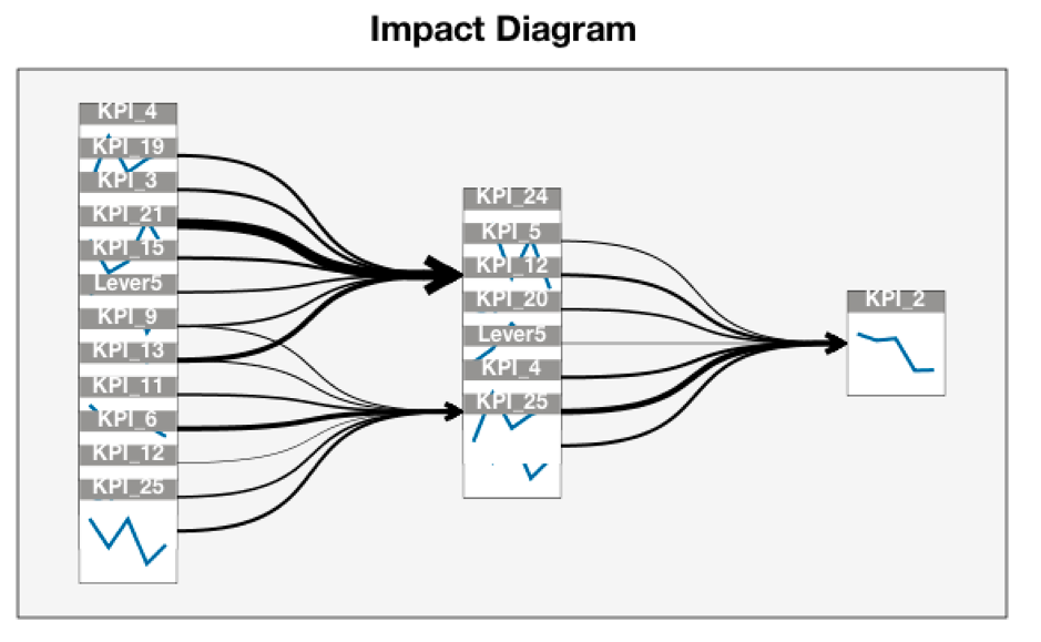 Alex opens the chart by double clicking and wants to see the detailed impact diagram. There is another chart displayed with 3 settings, "Series of interest", "Causes or Effects of the series" and "number of levels to display". From the Statistics help document, Alex gets the information that the series affecting the "Series of interest" are referred to as causes. The first level is just the series of interest. Each additional level shows more indirect causes or effects of the series of interest. He sets the "Number of levels to display" to 2, now, the impact diagram is updated. In this chart, the impact predictors are the ones selected in the TCM model. From this figure, KPI_4(sales) has the strongest impact for the target KPI_2(profit) because a smaller significance level indicates a stronger connection.
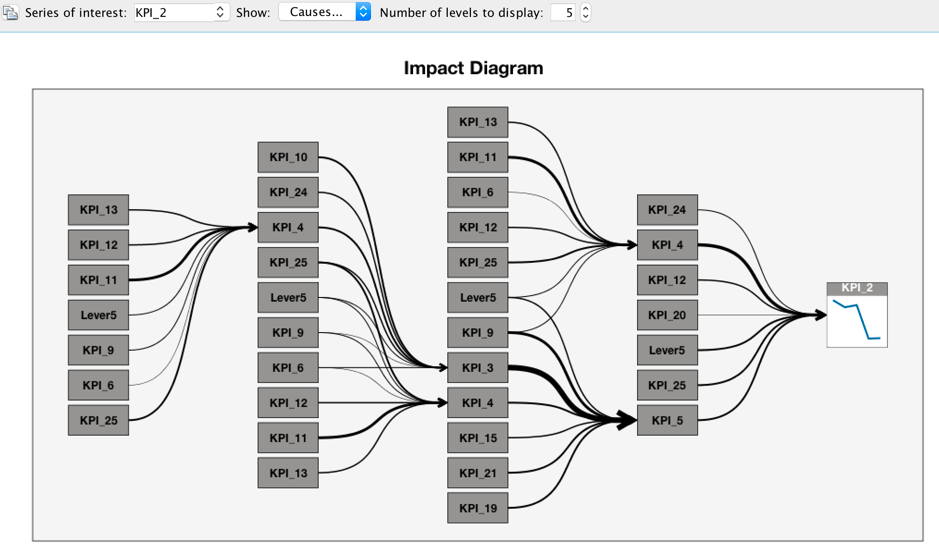
 When he sets the "Number of levels to display" to 5, more impact predictors are shown. It is important for a decision maker to consider all the potential causes together.
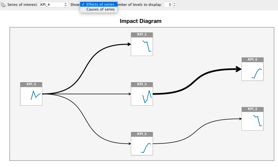
On the other hand, Alex wants to know what kinds of series KPI_4(sales) will effect. He specifies the "Series of interest" to KPI_4 and chooses "Effects of series". The impact diagram is changed to another format. From this chart, Alex draws a conclusion that the KPI_4(sales) will affect KPI_2(profit), KPI_5, KPI_3 directly.
Up to this point Alex has obtained the answer to his two questions by using the IBM SPSS TCM algorithm. He discovered all of the causal relationships among all of the time series he was interested in and found all of the potential impactful predictors for the target. Alex has found that KPI_4(sales) and KPI_25(cost) are important predictors for the target KPI_2(profit). One problem he sees coming is how KPI_2(profit) will change with KPI_4(sales) and KPI_25(cost). IBM SPSS TCM provides a scenario analysis feature to perform this kind of What-If analysis. In the real world, there are many anomalies in a large set of interrelated operational metrics. How is one to deal with it? An outlier detection approach is available for discovering all of the possible anomalies and the most likely root causes of the anomalies. These powerful features will be introduced in the next blog.
Where can you get the SPSS TCM?
Product Integration with UI
Harvested in the Product
- IBM Watson Studio, all the SPSS algorithms are available in the Watson Studio (DSX). When, using it follow the Watson Studio (DSX) access policy.
API Documentation for Spark and Python
- You can get the API Documentation for Spark and Python Here.
Based on the current design, before running TCM, the data must be prepared to a suitable format. Another SPSS algorithm named Time Series Data Preparation(TSDP) is used to do this, which makes the input data more structural and cleaner. After the TCM prediction, there is another SPSS algorithm named Reverse Time Series Data Preparation(RTSDP) to convert the prediction data used in TCM to have the same structure as the input data. The basic functions of TSDP include Group, Aggregation/Distribution and Missing Value Handling, which are not in the scope of the current blog. TSDP and RTSDP are designed to be embedded with TCM in IBM SPSS Modeler and Statistics, while in IBM Watson Studio, the TSDP and RTSDP are two independent services; they must be invoked separately.
Notebook
I also wrote a notebook using Scala for this use case, you can try it in the IBM Watson Studio .
#Statistics
#GlobalAIandDataScience#GlobalDataScience