Introduction
The amount of real-time data that is generated from users is enormous and thanks to science and technology which made it is possible to analyze, learn and predict using past data. It clearly resulted that with more data deep learning can give better results than machine learning techniques. Deep learning is an extension of machine learning and it is built using neural networks. The idea of neural networks was inspired by the central nervous system (CNS) present in the human brain where each neuron in the system shows reflexes and triggers the brain to take action from the outside world.
To build an intelligent system, the neural network has to learn from past data and remembers it in the form of weights. During model learning, we use several optimizers to understand the patterns from the data and adjust these weights in a way that the model gives minimal loss. Using optimizers and performing hyperparameter tuning we can improve the efficiency and performance of the model. Below are a few ways to improve the deep learning model:
Adding layers
Increasing no of neurons in the hidden layers
Changing activation and optimization fxn’s
Altering learning rate.
Activation Fxn's
Activation functions are non-linear in nature which allows for the approximation of complex functions and provides non-linearities into the network. The mathematical equation is given as Y’ = g (Wo + Xt * W) where Y’ is the predicted value, Wo is the bias value, Xt is the Transpose of input matrix X, W is the weights assigned and g is the activation function. Let’s see a few examples of activation functions
- Sigmoid Function: This function is an S-shaped curve ranging from (0-1). This function is defined as the ratio of unit value to the sum of the inverse exponential of input value x and unit value. This is one kind of non-linear function and is mainly seen in logistic regression in machine learning concepts. TensorFlow - tf.math.sigmoid(x)

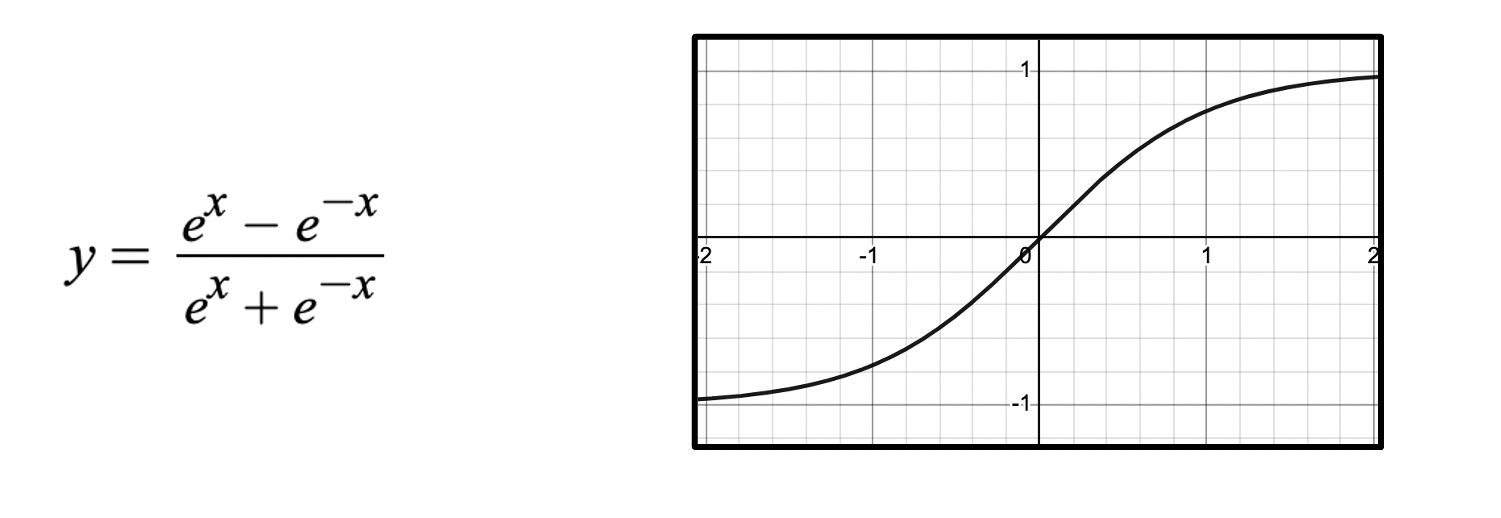
- Hyperbolic Tangent: This function is also a type of s-shaped curve like a sigmoid with a left-shifted position. This function comes under nonlinear functionalities. TensorFlow - tf.math.tanh(x)
- Rectified Linear unit (ReLu): This is the widely used function in the real time implementations. It is defined according to interval basis, Y=0 (where x<0) and Y=X(where x≥0)


Hyper-parametric tuning is the process of improving the neural network by adjusting the weights from the training data. There are many parameters that are involved in any kind of neural network. Below are few important (Hyper_parameters) listed :-
- Adding layers and increasing no of neurons.
- Change activation and optimization functions.
- Alter the learning rate.
- Increasing data.
The above are the ways to improve any deep learning model. As we have seen what are activation functions in the above sections, let's see where they can be used. Activation functions are used to help the network handle complex data and make helps in better learning. Now let's look into optimizers and the process of optimization in deep learning.
Optimization
Optimization is the process of analyzing the predicted results by looking into the loss value and improves in every iteration step. This is one of the major step to make model perform better and optimizers help achieving. There are many optimizers mainly concentrating on the concept called gradient descent. Few gradient descent functions are
- Stocastic Gradient Descent (SGD) [ tf.keras.optimizers.SGD ]
- Adam [ tf.keras.Adam ]
- Adadelta [ tf.keras.Adadelta ]
- Adagrad [ tf.keras.Adagrad ]
- RMSProp [tf.keras.RMSProp ]
All the above mentioned optimizers are built on the basis on gradient descent algorithm. Lets deep dive into the concept of gradients and how it is related in optimizing the model.
Gradient
Gradient is a vector of partial derivatives of each dimension and measures the steepness of the line. For any derivational equation in the 3 dimensional space, a gradient vector can be calculated at every point in the space. Let's look into a mathematical example.
Q) Find the gradient vector and maximum directional derivative at point (1,1) for equation F(X, Y) = 2X2 + 3XY + 4Y2.
∇ F(X, Y) = <∂F/∂X , ∂F/∂Y>; ∂F/∂X = 4X + 3Y; ∂F/∂Y = 3X + 8Y
∇ F(X, Y) = < 4X + 3Y, 3X + 8Y >
@ point (1,1): < 4(1) + 3(1), 3(1) + 8(1) >
∇ F(1, 1) = < 7, 11 > ( This is the gradient/vector. i.e, 7Î + 11Ĵ )
Maximum direction = √ (∂F/∂X)2 + (∂F/∂Y)2 = √ 72 + 112 = √170.
When the gradient is calculated, the vector represents the direction to travel for reaching the global maximum in the equation. In general, if you stand at point (X0, Y0, ......) in the input space of F, the vector ∇ F ( X0, Y0, ......) tells you which direction you should travel to increase the value of F most rapidly. This method is called Gradient ascent. In deep learning, our aim is to find weights that gives global minimum loss value. To achieve this we use gradients and go opposite to the direction that pointing which results in getting least possible loss and consider the weight associated in the function.
Let's see the algorithm of gradient descent.
Algorithm:
- Initialize weights randomly.
- Loop until convergence:
- Compute gradient: ∂J(W) / ∂W.
- Update weights: W <− W <− (η) × ∂J(W) / ∂W.
- Return weights.
η is defined as amount of step to be taken in the opposite direction of our gradient. η (eta) is known as learning rate. Small learning rate converges slowly and can stuck into false local minima. Large learning rates overshoot by taking large steps which becomes unstable and diverge. Stable learning rates converges smoothly and avoid local minima. For each iteration it takes certain step and tries to reduce loss as update in weights during loss optimization.
This is how optimizers and Activation functions are used and plays vital role in building a strong neural network model. It is important to make sure that the model shouldn't overfit while training the model. So we use regularlization techniques to make sure it won't either underfit or overfit. There are other important concepts like back-propagation and learning rate which plays major role in building the network.
We have come to an end to this article.
Follow my LinkedIn and Medium page for more updates on ML & DL.
Happy reading...! 📚 😁.