Weighted Idle governor

Author: Pratik Rajesh Sampat

Background

Efficient management of energy is an essential requirement for most of the systems. Modern processors provide a wide range of sleep states that allow different levels of energy savings. These idle states consist of two major properties:

Target residency - Minimum time to be spent in this state to save energy

Exit latency - Time taken to exit the idle state

Choosing a state that is too shallow hurts energy savings, while choosing a state too deep not only hurts energy savings but also incurs latency-residency penalties hurting performance.

Linux® provides CPU-idle governors to identify the idleness of a CPU and send that CPU to an idle state to save energy. Governors first attempt to quantify events that are more likely to be deterministic (such as timers) and then attempt to identify the next wakeup event based on the other non-deterministic events (such as interrupts in particular).The timer events oriented (TEO) CPU idle governor is a relatively new attempt to improve CPU-idle management while improving from the predecessor menu governor.

The timer-events-oriented (TEO) governor

The timer-events-oriented (TEO) cpuidle governor is a relatively new attempt to improve CPU-idle management while improving from the predecessor menu governor.

The TEO governor's working is based on the following principles:

The idea is that the timer events are the most likely source of wakeup. This is based on the observation that timers are at least two orders of magnitude more frequent than any other events on most systems.

It also introduces the concepts of early hits when a state is missed for the state that actually matches the measured idle duration.

Lastly, it also maintains a recent idle-time history interval to determine if majority of the idle durations are below the target residency to recompute a new expected idle duration. This is done to quantify non-deterministic events.

Figure 1. Illustration of the timer and buckets component

Figure 2. Recent idle-time history buffer

In this post, we are more interested in quantifying non-deterministic events. Therefore, the recent idle-time history algorithm is expanded to gain better understanding as follows

Follow a mechanism for pattern detection of non-timer wakeup sources

In a circular buffer, consider a number of intervals (around 8) into account.

Have a count of the intervals that are lesser than the current expected idle duration

If a majority of these are lesser, compute the average interval time for the buffer

Using the new-found interval time, find a shallower state matching the target residency.

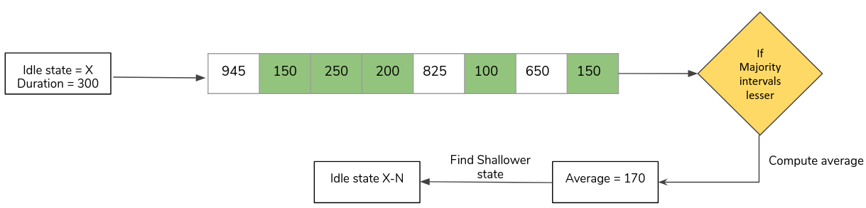
Figure 3. Example illustration - Recent idle-time history buffer algorithm

Is more history better?

This section further explores the recent-idle history duration and attempt to highlight the need for an alternate approach for gathering and using history for non-deterministic events.

This linear window approach to determine the expected value is light weight and often works quite well. However, can it be made better?

One straightforward approach that comes to mind when asked to improve the recent-idle window algorithm is to increase the window size. Therefore, the question that the section tries to answer: Is more history better?

Perform the following settings for the experiment:

Exponentially increase the size of the recent idle interval buffer from 8 to 128

Use the Schbench benchmark, which provides latency statistics for scheduler wakeups (i.e non-deterministic event), and worker threads are treated as the varying parameter

Metric of measurements
- Performance - latency 99th percentile - usec
- Power - watts

Performance and Power statistics are normalized

Let's first have a look at how latency is affected when the interval buffer size is increased.

The latency comparisons for different interval sizes is a mixed bag of numbers for each thread. Some interval sizes perform better for some thread scenarios and while some perform considerably worse.

A standout observation here is that the 128 latency intervals consistently perform better in terms of latency.

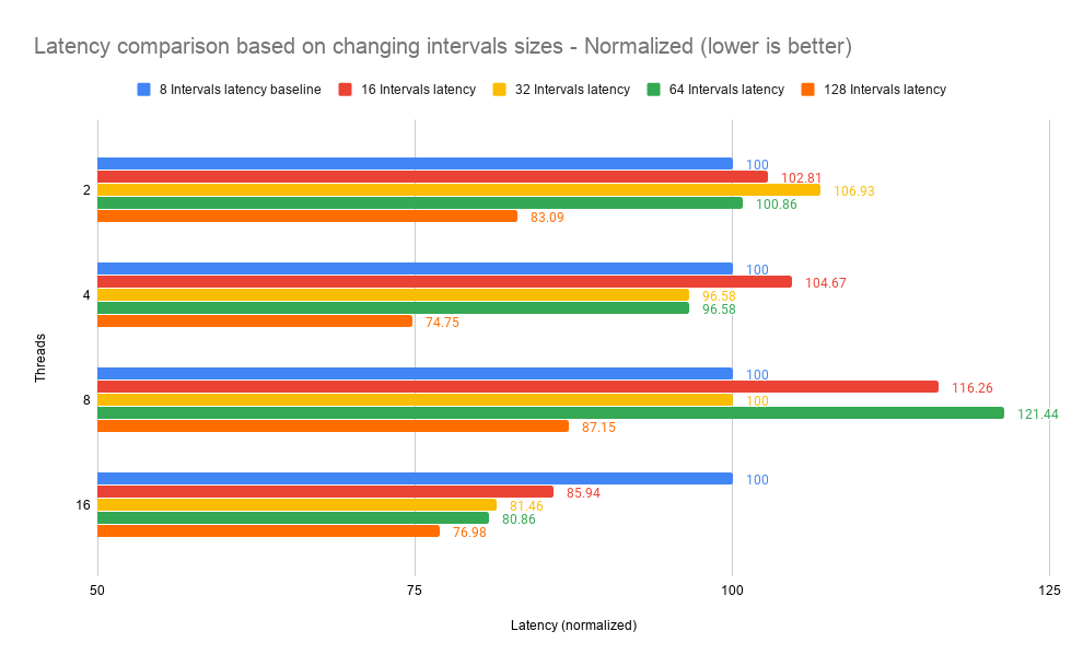
Figure 4. Latency comparison based on changing interval sizes

However, on comparing the energy consumption, it becomes clear that the power statistics are considerably worse for almost all the cases.

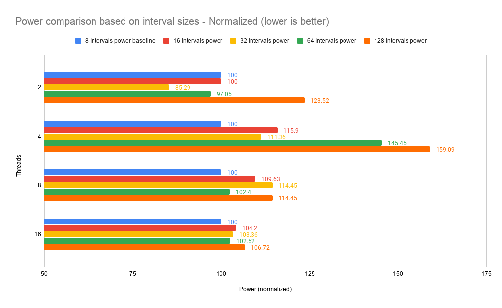
Figure 5. Power comparison based on interval sizes

You can infer the following information from the experiments conducted:

Shallow states are being more preferred with the increase in window size, hence reducing the latency and helping performance. However, this impacts energy savings considerably which is undesirable.

The current history mechanism is limited due to its linearity. Also, average of interval durations may not be a good metric when the distribution of data presents skewness

This seems more evident with the observed behaviour of increasing the interval window that the stale past may taint future predictions.

Therefore, a metric of measurement is needed that could account for both more as well as less recent history of idle durations without presenting skewness, while adapting to dynamic workloads to choose the correct idle state more frequently. Hence in the next section, an alternate mechanism of gathering history is presented based on probabilities that can ascertain the next idle state with a degree of confidence.

Weighted History Algorithm

The proposed algorithm is designed to store information about previous idle durations without the need to store raw idle-time data, as that could be cumbersome as well as when used with a metric of arithmetic mean would amplify skewness. Therefore, the probabilistic method to maintain history supplements the current cyclic idle history algorithm.

There are two main components of this algorithm. One is the technique to gather history and another is the method employed in using this gathered history.

Gathering History

The data structure is in the form of a matrix which describes the probability distribution (weights) of occurrence of each state per CPU

Each row signifies the distribution for that state, and the sum of the weights is always equal to 100

Each entry in the r (row) × c (column) matrix signifies the likeliness of occurrence of waking up with c’s residency when entered in idle r

Consider the following example of N idle states pre-populated with probabilities, wherein the summation of the weights that hold the probability = 100

When the idle governor chooses to enter idle state 2, the matrix lookup on that row exhibits the probability of occurrence of all the possible states determined by the past wakeup residency of the respective states.

For example, the state[2][1] = 0.55 and state[2][2] = 0.20 means that when state 2 has been picked by the governor, it would be a wiser decision to rather go to state 1 in order to achieve maximum performance per watt.

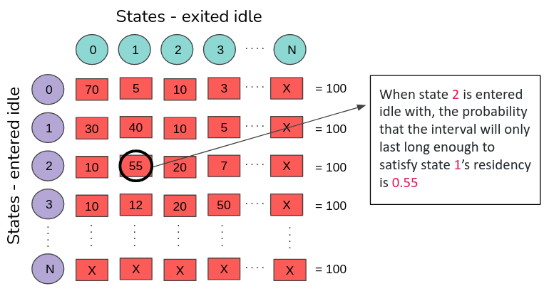
Figure 6. Sample probability distribution of idle states

Utilization of History

This section describes how probability weights are initially populated and how this metric is used to determine the next idle-state to enter.

A. Initialization of the data structure:

In the beginning, the states have higher probabilities for themselves.

The rest of the states are divided equally in probability summing up to 1 * scaling factor (in our example case 100)

Example: Assume that there are four idle states. The initial probability of occurrence for a state to occur when the initial predicted state is equal to the final entered state is 70%. Then the rest of the states have probability: ((100 - 70) / N -1) %

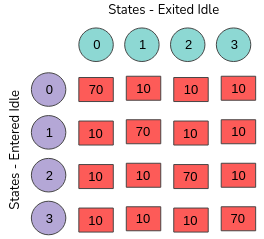
Figure 7. Initial probability distribution for idle-state occurrence

B. Learning from successes and failures:

The distribution of probabilities is dynamic, based on the kind of the workloads run

During retrospection, the correctness of the prediction is determined
- If the prediction was incorrect, the predicted state’s probability is reduced and that of the state which it should have rather gone into is increased.
- If the prediction was correct, the predicted state’s probability increases while the rest of the states reduces in equal proportion

The amount by which the weights must be increased or decreased is called the learning rate. The rate of learning can be static or dynamic

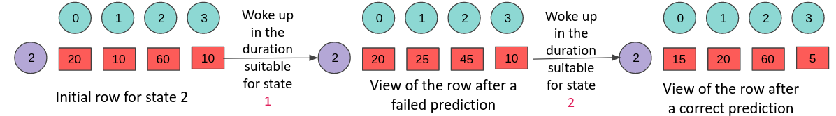
Figure 8. Example for weight correction based on correct and incorrect predictions

C. Prediction of the next state

The selection of the next idle state is based on probabilities, for which a biased random number generator is used

The biases of the generator comes from weights that are attached to each state

Naturally, a state with high probability is more likely to be chosen

For example, assume that the governor with the rest of its metrics has predicted state 3 and the probability weight distribution is as in Figure 9

The probability distribution for state 3, which is a list that holds the summation of the previous states, is maintained. In this case: wt_list[] = {12, 19, 64, 100}

A random number is generated and is multiplied by the scaling factor. For example, 0.6 * 100 = 60

The list is iterated until rnd_num < wt_list[idx]. In this example idx = 2.

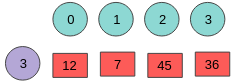
Figure 9. Illustration of picking the next idle state

This raises a question of why don't we just pick the state with the highest probability instead?

In case of multiple states closely competing for dominance, having a scheme to pick a state with the highest probability may not always be correct

Although it is evident that the algorithm will self-correct itself, the behavior of the workload may have changed and hence in such a case, the algorithm will always be left playing catch-up.

If multiple states are close in probabilities competing for dominance, then there should be a fair chance for each of the competing idle state to be picked. This helps to ensure better accuracy.

For example, let's consider the following state distribution:

If gone by the highest probability strategy, state 0 will be picked

However state 2 and 3 were also very close in terms of likeliness to have be correct

Once woken up correction can be applied

However, if the weight distribution pattern exhibits contention between multiple states often; then we would be left playing catch-up

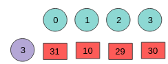
Figure 10. Illustration of idle contention

Results

Setup

To evaluate the initial performance of the weighted TEO governor, an IBM® POWER9™ processor-based server is employed, with a two-socket machine of 16 cores each. The memory on the system is 1 TB. The machine runs Ubuntu 16.04 with modified 5.6 kernel.

Metrics of measurement

Performance (latency / throughput)

Power (watts)

Accuracy
- Correct prediction - The idle state predicted aligns with the actual sleep duration
- Undershoot prediction - The actual sleep duration is shallower than the idle state predicted.
- Overshoot prediction - The actual sleep duration is deeper than the idle state predicted.

All the metrics of measurements are normalized.

Based, on the above setup and the metrics of measurements, the algorithm is run of two benchmarks schbench and pgbench

Benchmark: Schbench

Benchmark provides detailed latency distribution statistics for scheduler wakeups. The varying parameter in the experiment is worker threads. Scale of measurement:

99th percentile latency - Normalized

Power - Normalized

Both lower values are better

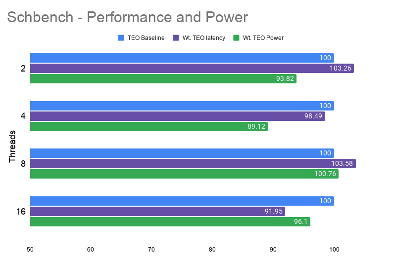
Figure 11. Schbench - Performance and power comparison for varying threads

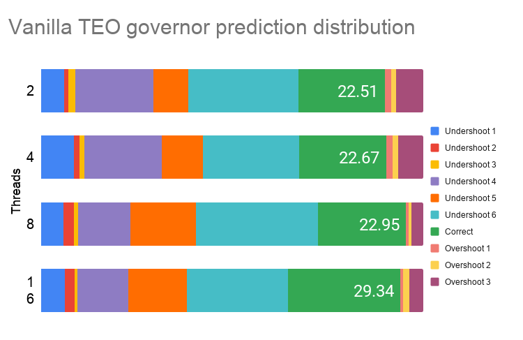
Figure 12. Schbench – idle state prediction distribution for vanilla TEO governor

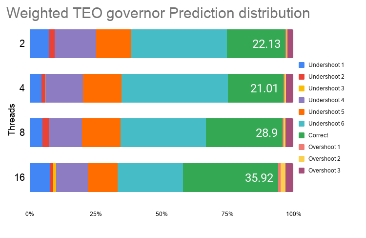
Figure 13. Schbench – idle state prediction distribution for weighted TEO governor

Observations:

Performance shows improvement of ≈8% with maximum regression of ≈3%

Power shows maximum improvement of ≈11%

Accuracy of predictions shows maximum improvement of ≈46%

Benchmark: Pgbench

Benchmark is a simple program for running benchmark tests on PostgreSQL. It runs the same sequence of SQL commands over and over, possibly in multiple concurrent database sessions, and then calculates the average transaction rate. Scale of measurement:

Number of transactions - Normalized - higher value is better

Power - Normalized - lower value is better

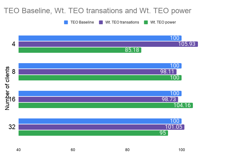
Figure 14. Pgbench - Performance and Power comparison for varying threads

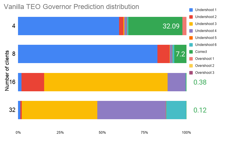
Figure 15. pgbench – idle state prediction distribution for vanilla TEO governor

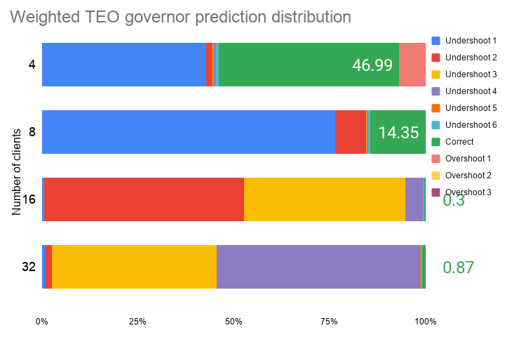
Figure 16. pgbench – idle state prediction distribution for weighted TEO governor

Observations:

Performance shows improvement of ≈5% with maximum regression of ≈2%

Power shows maximum improvement of ≈15% with maximum regression of ≈4%

Accuracy of predictions shows maximum improvement of ≈14%

Conclusion

The proposed solution of weighted randomization does show promise in increasing the accuracy of prediction of the idle states based on their residency and thus in turn improving both tail latencies incurred on wakeups and energy consumption for the overall system. Initial results show that this solution helps increase accuracy by ≈46% while improving on performance (latency / throughput) by ≈10% and improving energy consumption by ≈15%, and therefore, also displaying a strong correlation between accuracy and performance-power metrics.

The preliminary results on benchmarks present a view of an alternate approach for quantifying non-deterministic events in the operating system, keeping in mind the need for a lower CPU-intensive mechanism while increasing accuracy in idle-state management.

Although this method is based on probabilities as a mode of statistical measurement, the weights can still become stale and past trends can taint future predictions. It is necessary to devise an aging mechanism that can decay the weights over time to consider only the relevant information. The rate of decay is an area that needs to be further evaluated.

Moreover, properties such as rate of learning need to be evaluated for their optimal value or designed to achieve optimality over the course of decision making, and such a model should also be verified experimentally and mathematically.

Enterprise Linux

Weighted CPU-Idle governor

By Pratik Sampat posted Fri March 05, 2021 05:50 AM

Weighted Idle governor

Author: Pratik Rajesh Sampat

Background

The timer-events-oriented (TEO) governor

Is more history better?