Context
The IBM Data Science Elite (DSE) is a team of data scientists and data engineers who work with a select group of IBM clients to test and implement data science solutions — at no additional cost to those clients. The DSE team is the result of a stark reality that companies need to add data science to their fundamental business processes, but often struggle to proceed on their own. One of IBM's clients, a large supply chain company, worked with the IBM DSE to see if they could help predict their employee churn.
We'll walk you through the business case and conceptual underpinnings of the modeling prior to talking about exactly what we uncovered. To respect the client's privacy and corporate policies, some of the examples will use fictional features, but all are are meant to be illustrative and will be noted throughout the text. As a result of the modeling, the client would be able to recoup nearly $5 million in annualized cost.
Business Case
There's no company today that can avoid the fight to retain the best talent within their organization. Employee churn is a costly problem as employees are expensive to find and retain; both in terms of time and capital. The costs of losing talent are generally well documented, and for the client specifically, they include lost productivity of new employees, on-boarding and training costs, negative cultural impacts, lost knowledge, decreased team member engagement, and the time spent hiring new employees. With company culture and employee welfare being so important to our client, they needed a plan of redress.
Companies like this supply chain corporation may have turned to data science to understand churn broadly, but in applying those practices on internal operations, they can fundamentally change their business and do things like identify patterns in the behaviors of employees who might leave. If they succeed in predicting whether an employee is likely to churn, they can be proactive in addressing the potential causes so as to minimize the cost of replacing them.
IBM and the client used 5 years of anonymized employee data as the basis for identifying the patterns of churn of sales representatives. With rising rate of turnover and a tightening labor pool, their mission to decrease the loss of sales specialists was critical for the future of their business.
Models Tested
In the process of selecting models for a data science project, it is best practice for a data scientist to evaluate models sequentially. Models that offer the greatest parsimony are preferable, so begin with them and then compare those against models of greater complexity. The easier it is to explain the effects of the inputs on the ultimate output, the more easily the business can adapt its behavior being measured to strategically align with the inputs of the most desired output.
In this case, the goal of the project was to classify whether an employee would, or would not, churn. In the IBM Data Science Elite engagement they tested logistic regression, random forests, and boosted trees to see which was the most accurate classifier. For the client, parsimony is attractive here because you want to easily describe the parameter effects that result in losing your top talent so you can address those problems. Logistic regression was tested first and offers much by way of explainability, so let's contextualize it first.
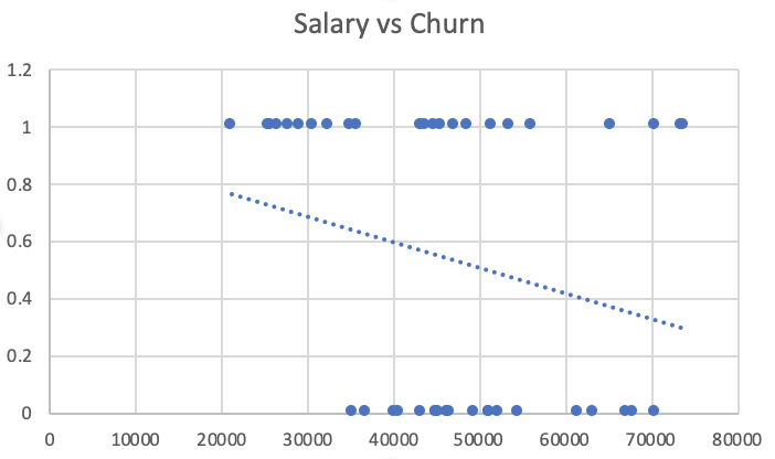
wherein some independent variable linearly predicts a quantitative value of our interest. We want to find the weight of the effect of that variable ( β1 ). You might reasonably guess the above model would struggle to predict attrition with historical example labels of 0 or 1. That's because we will run into a problem where our model predicts values in either the negative range or range greater than 1. This is observable in the figure below in the assumed continuation of the fitted line; somewhere close to $100,000 predicted values will turn negative (note these are fictionalized data points used only as exemplars). In the case of classifications, that result set doesn't make sense. We only want to see 1 (whether they will churn) or 0 (whether the will not churn).
Logistic regression by comparison constrains predictions between two values 0 & 1 while taking in the same input, X. The output changes with logistic regression. We're no longer predicting some scalar value, but are instead predicting the probability of the outcome occurring - whether we will or won't see employees quit. You'll notice the parameters, or weights, of the linear regression model (1.1) looks very similar to the weights in our logistic function (1.2).
p(X) = e^(β0 + β1X)/(1 + e^(β0 + β1X)) (1.2)
Those coefficients are estimates with a range of certainty, and as data scientists we can use them to intuitively and precisely to understand the relationship between or independent and dependent variables. Again, this is one of the most obvious benefits of logistic regression as a classification model. Its weights offer much parsimony, i.e. the ability to explain what drove the prediction within the model. There are many predictive modeling exercises where that simplicity has intrinsic value, and the employee churn use case is an obvious one. If we can easily attribute and communicate what is driving employees to leave, then we can address that underlying cause!
Random forest, was the next model tested. It is an algorithm designed to be a departure from the linear models discussed above. Namely, if the underlying relationship between predictors and response is complex and clearly non-linear, it's fair to presume the tree-based methods may catch more of the signal than strictly linear models. Let's again give it a small bit of theoretical context (random forests are designed to account for the weaknesses of decision trees).
Regression/decision trees are a fairly intuitive model design with some nice qualities in terms of explainability. The intuition behind regression trees is to segment samples into stratified groups based on values in the features that offer the cleanest segmentation. In the case of this client, if we imagine that we had the (fictional) features RecentManagerRating, CoworkerApprovalRating, and MonthSincePromotion to predict the salary of their employees, the decision tree might look like Figure 2.
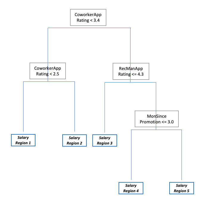
Each of those splits (starting with the fictional CoworkerAppRating, 3.4, at the top) are made upon the values which offer the greatest possible reduction in the difference between the predicted value and the mean value from the training data. In other words, the training data is split on CoworkerAppRating 3.4 because when you take the mean salary of the training samples with rating 3.3 or less, and the mean salary of training samples with 3.4 or more, and compare each respectively with the predicted value, it minimizes your error.
Ultimately, the data is segmented up in the above fashion until some stop condition is met. There’s then some pruning of leaves on the tree, but that is the essence of the approach. This modeling process can be quite powerful, but also problematic when it comes to a trade-off between bias and variance. Regression trees suffer from high variance — flexing and changing much with the training data provided to the model.
Random forests are a progression from decision/regression trees designed to speak to those weaknesses. Many of the principles of fitting random forests appear familiar to that of fitting regression trees (making splits on variables of importance), but here fitting many trees instead of one. Additionally, the process differs by using bootstrapped training data on those trees (which just means creating new sample sets from the original data set by continuously randomly selecting samples). The main difference, and the crux of the random forest, is that at each split in the tree, only a randomized subset of the features (e.g. Coworker Approval Rating and Months Since Promotion, but not Manager approval rating) are available for the model to consider. Only having a predictor subset de-correlates the many trees trained, and so the resulting trained trees are much more reliable. Lastly, average of the predictions is then taken from those many trees or, in the case of classification, such as whether an employee will leave, we simply take a majority vote of class predictions from each of the trained trees.
Ultimately, the client and the IBM Data Science Elite tested both models, but settled on a model derived from the concept of a boosted tree - XGBoost.
Models Chosen
The model chosen by the IBM Data Science Elite team to gather the most signal from the client's data was XGBoost. The intuition behind XGBoost is best explained through the concept of Boosting generally and its design becomes more easy to understand when compared with the Decision Trees and Random Forest explained above.
Boosting looks similar to Random Forests in that there are many trees trained on an original data set (in this case the data set is modified rather than bootstrapped). In boosting, however, training each tree does not happen independently of all other trees. Each tree is trained using information from the tree before it - trained on the weaknesses of the tree trained before it.
The trees are trained sequentially. For example, using our fictional features from our client, if your first tree had residuals (differences between the predicted value and the training value) because it missed on a split made on Manager Approval Rating, those residuals are used as input in training on the tree subsequent to it. This system of training trees that have to account for the failure of their predecessors may sound slow, but that’s the intent. Train many small trees slowly. It prevents overfitting to your training data, and by extension it earns your model some extra signal. XGBoost is a specific implementation of the more general concepts behind boosting. If you understand the intuition above, you can reasonably discern the overall process for XGBoost.
In the case of the supply chain company and the IBM Data Science Elite, XGBoost achieved 86% accuracy in classifying employee churn cases. Classification accuracy in this case has a very specific meaning and is defined as the ratio of True Positive and True Negative to the full set of Positive and Negative.
Accuracy = TP + TN / (TP + TN + FP + FN)
This was a significant achievement for the client team in terms of designing and developing retention plans for their employees that were valuable to their company. With IBM's help, they were able to identify patterns of employees likely to leave and address the underlying factors. The top three features most indicative of people leaving:
By designing retention plans with these key features in mind, and presuming only an improvement of 20% in the retention rate for the client's sales staff after adapting these plans, they stand to save close to $5 million annually. Ingraining data science into daily operations fundamentally changes how businesses operate and provide the differentiator to carry them into the future. IBM excels in these use cases which make a difference for enterprise clients.
Summary
The IBM Data Science Elite and supply chain client engagement was an incredible opportunity to partner together to solve an enterprise problem of critical value. The steps dictated above are a useful conceptual walkthrough, but not entirely comprehensive of a data science solution. Keep in mind that the DSE team also spent significant time and investment in cleaning and preparing the data, as any team would in order to build effective and powerful models. Additionally, if the models are to drive value for an enterprise, they need to be deployed and accessible. A report with the feature importances and model chosen is valuable, but a model made available for consumption over REST to predict whether an employee is soon to leave allows management be proactive in working with those employees.
If you're curious to learn these concepts more in depth, consider registering for the IBM Data Science Community to be kept up to date with all the content published there. Additionally, I'm constantly reviewing the many resources that have helped teach me data science — I've included each and every one I reviewed to fact-check and refresh myself for this article.
Stack
For the engagement the IBM Data Science Elite used: - Watson Studio Local
References
#Hands-on
#Article#datascience#DecisionTrees#DSE#GlobalAIandDataScience#GlobalDataScience#Hands-on#Jupyter#LinearRegression#LogisticRegression#MachineLearning#ModelSelection/HyperparameterTuning#Notebook#Python#SVMs#Tutorial#UseCase