For decades, statistical theorists have debated the merits of the classical or frequentist approach versus the Bayesian approach. Googling Bayesian versus frequentist produces a vast collection of items on this topic. Even XKCD has weighed in (
XKCD). (But see also this link for a vigorous debate on this:
What's wrong with this?). Applied statisticians, though, have until recently been overwhelmingly in the frequentist camp.
There are, I believe, three main reasons for this.
- First, and possibly due to the next two reasons, applied statistics courses have mostly not spent much time on Bayesian approaches.
- Second, Bayesian methods require a prior distribution to be specified for the parameters to be estimated. While these methods work very well when there is prior information, often in applied work there is little such information available.
- Third, and perhaps most important, there has been a dearth of efficient, easy to use, mainstream statistical software for Bayesian analysis.
Why should you be interested in Bayesian methods? After all, Bayesian methods often give similar results to classical methods. Well, one nontheoretical reason is that Bayesian methods are hot right now! You might want to jump on the bandwagon. More serious reasons include these.
- Bayesian methods provide a rigorous way to include prior information when available compared to hunches or suspicions that cannot be systematically included in classical methods.
- Bayesian methods provide exact inferences without resorting to asymptotic approximations.
- Bayesian results are easier to interpret than p values and confidence intervals. They allow us to talk about results in intuitive ways that are not strictly correct with classical methods. I will show an example below.
- Bayesian results show the whole distribution of the parameters rather than just point estimates.
The New Procedures
Among the last things I did before retiring from IBM at the end of 2015 was to create four Bayesian extension commands which are available via the Extension Hub from within Statistics 24 or later or via Utilities in older versions. IBM SPSS Statistics version 25, though, introduces seven native Bayesian procedures in nine dialog boxes. They have the familiar Statistics user interface style, have traditional Statistics syntax, and, like other procedures, produce tables and charts in the Viewer. They are included in the Statistics Standard Edition. The
Analze > Bayesian Statistics submenu lists the procedures.
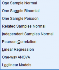
Figure 1: Bayesian menu
The commands are BAYES ANOVA, BAYES CORRELATION, BAYES INDEPENDENT, BAYES LOGLINEAR, BAYES ONESAMPLE, BAYES REGRESION, and BAYES RELATED.
Before we dive into the procedures, we need to address the second problem above where we don’t have a firm basis for selecting a prior. If we do have prior information, it can be valuable. We specify it in the prior. The procedures give a variety of choices, and that information will be combined with the data in the posterior distribution. But if we don’t, we might use a noninformative prior such as that all values are equally probable. As the amount of data increases, the impact of the prior on the posterior distribution, which incorporates both the prior and the data, is dominated by the data, so the prior choice becomes increasingly unimportant as long as the prior has positive probability for the relevant parameter space.
There are, however, difficulties with a uniform prior over an infinite space. Newer methods, referred to as reference priors provide a solution. The mathematics is beyond the scope of this note, but the important thing is that they allow us to have objective Bayes estimates. Reference priors are available in the appropriate procedures and are generally the default.
A Classical Versus Bayesian Test Procedure
I am not going to add to the many commentaries available on the web or in textbooks on Bayesian methods, but I will illustrate the approach and compare it with classical methods for the independent samples test for equality of means. The familiar classical test is on
Analyze > Compare Means > Independent Samples t test, and the Bayesian equivalent is on
Analyze > Bayesian Statistics > Independent Samples Normal.
Using the small data file creditpromo.sav shipped with Statistics and used in the independent samples t test case study, we will test whether the amount spent by store card holders differs depending on what promotion they received. (See the Case Study for details.) Our null hypothesis is that there is no difference. With the classical t test, we get this result (I have edited down some of the output.)
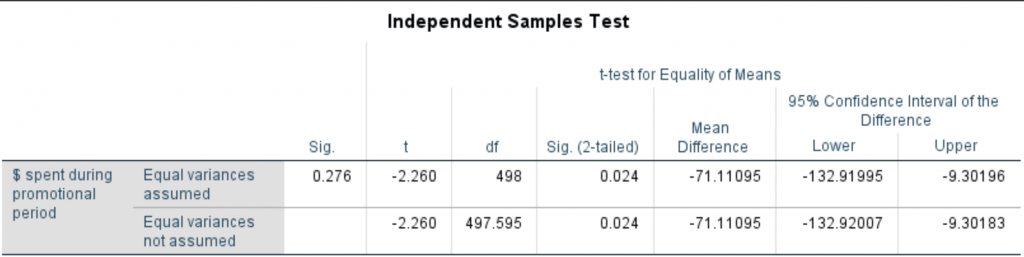
Figure 2: The t test output
The significance level, equal variance not assumed is 0.024 with a mean difference of -71.11 and a 95% confidence interval of (-132.92, -9.30), so using the traditional but arbitrary 5% criterion, we reject the null. In words, the probability of a difference of this or larger (absolute) magnitude is 2.4%, which is very unlikely, so we reject the null and accept the alternative. The p value is the proportion out of all possible samples that give an absolute difference at least this large under the null, although we have observed only one of these. And the confidence interval is the interval such that if we draw samples like this many times, the true difference will be in this interval 95% of the time. A bit tricky but familiar language. The true difference is a fixed value, not a random variable with a probability distribution, so we can’t make probability statements about it.
Now let’s do this the Bayesian way. The dialog box looks much the same as the t test dialog (not shown).
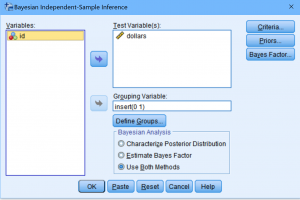
Figure 3: The Bayesian dialog
But we need to choose the prior. We will use noninformative priors for the mean and variance. This is some of the output.
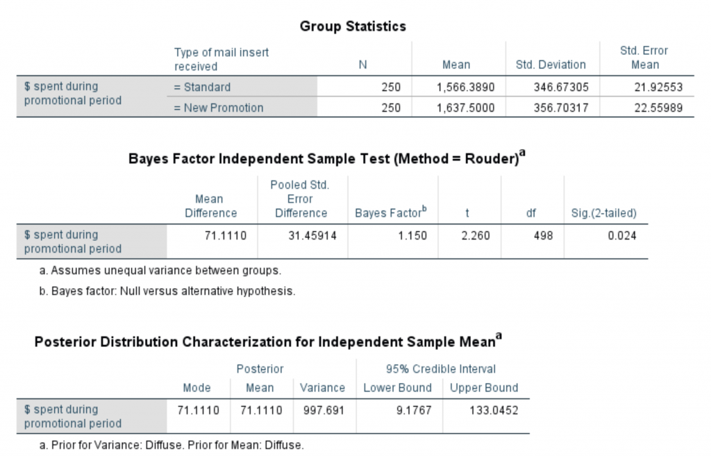
Figure 4: The Bayesian output
As you can see, we get the same test output, but we get two interesting different items. Instead of a confidence interval, we get a 95% credible interval, which has the interpretation we intuitively want: We are 95% certain that the difference in the means is between 9.177 and 133.045, which is slightly different from the confidence interval. (The signs are reversed, but this is arbitrary.) We can make a probability statement about the parameter values.
The other interesting statistic is the Bayes Factor, 1.15. It is just the ratio of the data likelihoods given the null versus the alternative hypothesis. So we can say that the null and alternative hypotheses are about equally likely. We don’t have a way to make a statement like that using classical methods.
Going further, as an additional output we can get a plot of the prior and posterior distributions. As you can see, the noninformative prior is flat. While the classical method gives us a point estimate of the effect (and a confidence interval), the Bayesian output shows the whole posterior distribution.
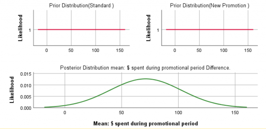
Figure 5: The priors and posterior distributions
If we have prior information available, this curve would change. Here are the prior and posterior graphs with a prior that might be based on previous experiments. It has a substantial effect since the sample size is small, but with more data, the effect of the prior would wear off.
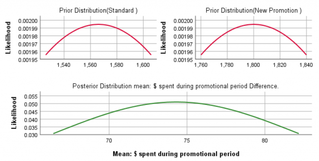
Figure 6: The posterior distribution with an informative prior
This note just scratches the surface. Bayesian methods require some study, but I hope this note has piqued your interest and that you will go further into this methodology. The Case Studies on the Bayesian methods may help get you started.
#bayesian#IBMSPSS#SPSS#SPSSStatistics